Empowering Pharma with Posit and Snowflake: From Raw Claims to Regulatory Insights


Pharmaceutical and life sciences organizations increasingly rely on real-world data (RWD) — electronic health records, insurance claims, patient registries, and digital health data — to generate real-world evidence (RWE) that complements randomized clinical trials. That evidence shows up across the drug lifecycle: health economics and outcomes research (HEOR), post-marketing safety surveillance, claims-based comparative effectiveness studies, and clinical trial feasibility assessment. Getting from a raw claims extract to something a regulator will accept as evidence is a long pipeline — cleaning and standardizing messy data, running the same repetitive analyses over and over, and proving every step is reproducible. This piece walks through where Posit and Snowflake fit into that pipeline, and — grounded in specific PharmaSUG presentations from teams at Pfizer, Merck, Graticule, and others — what people are actually building with the combination.
(Genomics, drug discovery, and gene expression analysis are also areas where the open-source R/Bioconductor ecosystem is heavily used in pharma, but that’s a different data and tooling story from the claims/EHR-driven RWE work this piece focuses on.)
A useful way to see what this looks like in practice, outside of any single vendor’s pitch, is a boutique RWD consultancy like Plinth, which builds its entire practice — cohort builders, Shiny dashboards, reproducible reporting pipelines — on R, Shiny, Posit Connect, dbplyr, renv, targets, and Snowflake (among other database backends), serving RWE teams at organizations like AstraZeneca, Flatiron Health, and PicnicHealth. R as the analysis layer, Shiny/Quarto for delivery, Snowflake (or another warehouse) as the data layer, all wired together for reproducibility — that’s the same general pattern showing up across the presentations below.
What “Posit Team” Is
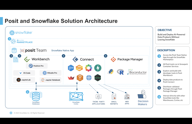
“Posit Team” is Posit’s bundling of three products that, together, cover the full loop from writing code to sharing results:
- Posit Workbench: a server-based environment where data scientists and biostatisticians work in their preferred IDE — RStudio, VS Code, or Posit’s polyglot IDE Positron — against shared compute and data access, rather than everyone working on separate laptops with separate package versions.
- Posit Package Manager: mirrors and pins CRAN, Bioconductor, and PyPI package versions, so a project’s dependencies stay fixed and reproducible over time — important when a study’s results may need to be reproduced or audited years later.
- Posit Connect: a publishing platform for sharing the output of that work — Shiny apps, Quarto reports, APIs — with people who don’t work in the IDE at all (reviewers, clinicians, project managers).
None of these three products require Snowflake specifically; they work with any data source. The Snowflake angle is about where the data lives and how compute reaches it.
Architecture: Two Ways Posit and Snowflake Fit Together
Posit and Snowflake support two different deployment patterns, depending on where the actual compute runs relative to the data:
flowchart LR
    subgraph OptionA["Option A: Posit inside Snowflake"]
        direction TB
        A1[Programmer's IDE] --> A2["Posit Workbench<br/>(running on Snowpark Container Services)"]
        A2 --> A3[(Snowflake Data)]
        A2 --> A4[Posit Connect<br/>Shiny / Quarto]
    end
flowchart LR
    subgraph OptionB["Option B: Posit outside Snowflake, connecting in"]
        direction TB
        B1[Programmer's IDE] --> B2["Posit Workbench<br/>(hosted elsewhere: on-prem, another cloud)"]
        B2 -- "OAuth, viewer identity delegation" --> B3[(Snowflake Data)]
        B2 --> B4[Posit Connect<br/>Shiny / Quarto]
        B4 -- "OAuth" --> B3
    end
Option A — Posit deployed inside Snowflake. Posit Team can run directly inside a Snowflake account via Snowpark Container Services (SPCS), installed as a Snowflake Native App. R and Python sessions execute on compute that lives inside Snowflake’s security boundary, so data never has to leave the warehouse to be analyzed.
Option B — Posit deployed outside Snowflake, connecting in. Posit Team runs on its own infrastructure — on-prem, another cloud, wherever it’s already hosted — and reaches into Snowflake as an external data source. Developers connect using OAuth with viewer identity delegation, so a query run from an interactive app or scheduled report respects the exact access control lists already defined in Snowflake’s own governance system, without shared service accounts or hardcoded credentials.
Both patterns share the same Workbench/Package Manager/Connect tooling; the difference is purely where the compute boundary sits relative to the data.
Push compute to the data, not data to the compute. Regardless of which deployment option is in play, the same principle that makes any database integration fast applies here: filter and transform as much as possible inside Snowflake, and only pull back the small result set you actually need to work with locally. In R, dbplyr translates ordinary dplyr verbs into SQL that runs inside Snowflake — a pipeline like filter() |> mutate() |> summarise() executes as a single pushed-down query, and collect() is the only point where data actually moves into R’s memory:
library(dplyr)
library(dbplyr)

# All of this executes inside Snowflake — nothing is pulled locally yet
t2dm_cohort <- tbl(conn, "PATIENT_DIAGNOSES") |>
  filter(diag_cd %like% "E11%") |>
  group_by(patient_id) |>
  summarise(n_diagnoses = n(), .groups = "drop") |>
  filter(n_diagnoses >= 2)

# collect() is the only step that actually moves rows into R's memory
t2dm_cohort_local <- collect(t2dm_cohort)
The same principle applies in Python, either through Snowpark’s DataFrame API (which compiles to SQL executed inside Snowflake) or a SELECT ... WHERE issued via a plain database connector before loading into pandas:
from snowflake.snowpark import Session

session = Session.builder.configs(connection_parameters).create()

# Filtering and aggregation both run inside Snowflake via Snowpark
t2dm_cohort = (
    session.table("PATIENT_DIAGNOSES")
    .filter("DIAG_CD LIKE 'E11%'")
    .group_by("PATIENT_ID")
    .count()
    .filter("COUNT >= 2")
)

t2dm_cohort_df = t2dm_cohort.to_pandas()  # only step that pulls data locally
Pulling a million-row table into local memory just to filter it down to a few thousand patients is the exact kind of latency and cost this pattern avoids — worth calling out explicitly, since it’s easy to write R or Python code that accidentally does the pull first and the filtering second.
Practical Workflows: What Teams Are Actually Building
The examples below are drawn from specific PharmaSUG 2025/2026 presentations. Some describe tools built specifically with Posit products; others describe general RWD methodology that this same stack is used to implement, without being tied to a particular vendor.
1. Bridging SAS and R at the Query Layer
Pfizer’s RWD programming team built an R function, sfcreate(), deliberately designed to mirror the structure of their existing SAS macro of the same name, so programmers moving from SAS to R don’t have to relearn a new mental model. The function also accepts SQL query text written with either SAS macro-variable syntax or R glue-style interpolation, as long as the corresponding variables exist in the R environment:
DBSTARTDT <- "01-01-2024"
DBENDDT   <- "31-12-2024"

# SAS macro-variable syntax, reused as-is from existing SAS code
sfcreate(
  name  = "enrolled_patients",
  index = "patientid",
  query = "
    select * from enrollment
    where claim_dt between date(&dbstartdt.) and date(&dbenddt.)
  "
)

# R glue-style syntax
sfcreate(
  name  = "enrolled_patients",
  index = "patientid",
  query = "
    select * from enrollment
    where claim_dt between date({DBSTARTDT}) and date({DBENDDT})
  "
)
This lets programmers reuse SQL logic that already exists in SAS macros without a full rewrite. The substitution itself is handled inside sfcreate() — plain R string literals won’t resolve SAS macro variables on their own.
2. AI-Assisted Table Generation
Pfizer’s RWD team also built RWD OR Output Chat, a Shiny application that uses an LLM with retrieval-augmented generation (RAG) to generate R code for their internal oroutput table framework (oroutput_prepfile(), oroutput_module(), oroutput_compile(), and oroutput_makeFormatWorksheet()) from natural-language requests. A few design details:
- When a programmer uploads a cohort dataset, the app reads its actual column names and includes them in the system prompt, so the LLM references case-sensitive columns correctly instead of guessing.
- Generated code lands in three editable boxes — Import Dataset, OR Output Functions, and Notes & Export — that the programmer reviews before running anything.
- For validation, the app opens a separate, freshly initialized LLM chat session with each called function’s actual source code loaded as context, and asks it to check the call against the real definition, rather than trusting the same conversation that generated the code to also grade it.
- The app never produces the final deliverable itself — programmers download the generated R script and run it themselves in their own IDE.
3. A Shared R Package + Shiny App for Routine RWE Analyses
Merck’s RWD programming team built an internal R package (and matching Shiny app, deployed on Posit Connect) called explorer, aimed at standardizing the repetitive analyses that come up in nearly every RWE study: Table 1 summaries, regression, Kaplan-Meier survival curves, meta-analysis, and classification metrics for comparing model or rule-based outcome definitions. R users call explorer::explore() directly; non-R users get the same functionality through the Shiny app’s point-and-click interface, so a single codebase serves both audiences.
One specific piece worth walking through is the classification-metrics module, which computes sensitivity, specificity, PPV, NPV, and F1 score for candidate rule-based outcome definitions against one or more reference (“silver standard”) columns:
cutoff_results <- reactive({
  data <- filedata()
  setDT(data)

  req(silverf())
  req(definef())

  defcol       <- scan(text = definef(), what = "", quiet = TRUE)
  outcome_cols <- scan(text = silverf(), what = "", quiet = TRUE)
  results_list <- list()

  for (outcome_col in outcome_cols) {
    for (definition_col in defcol) {
      metrics <- calculate_metrics(data, definition_col, outcome_col)
      if (is.numeric(metrics$sensitivity) && !is.na(metrics$sensitivity)) {
        results_list[[paste(definition_col, outcome_col, sep = "_")]] <- metrics
      } else {
        message(paste("Metrics for", definition_col, "using", outcome_col, "are invalid."))
      }
    }
  }

  results_df <- do.call(rbind, lapply(results_list, function(x) {
    data.frame(
      TP = x$TP, TN = x$TN, FP = x$FP, FN = x$FN,
      Sensitivity = x$sensitivity, Specificity = x$specificity,
      PPV = x$ppv, NPV = x$npv, F1_score = x$f1_score,
      stringsAsFactors = FALSE
    )
  }))

  if (nrow(results_df) == 0) stop("No valid metrics obtained; results_df is empty.")

  results_df <- cbind(metric_name = rownames(results_df), results_df)
  rownames(results_df) <- NULL

  results_split <- setDT(results_df)[
    , c("Definition", "Silver_standard") := tstrsplit(metric_name, "_", fixed = TRUE)
  ][, Standard := ifelse(duplicated(Silver_standard), " ", Silver_standard)]

  results_split[, c("Standard", "Definition", "Sensitivity", "Specificity", "PPV", "NPV", "F1_score")]
})
This is genuinely useful in RWE work: teams often build several candidate rule-based definitions of an outcome (e.g., “2+ diagnosis codes within 12 months” vs. “1 diagnosis code + 1 prescription”) and need to score each one against a trusted reference before picking which definition to use in the actual study. One thing to watch, if adapting this pattern: splitting metric_name on "_" to recover the original column names only works cleanly if those column names don’t themselves contain underscores — a real risk with typical database naming conventions (e.g., AGE_N, OUTCOME_CHART_REVIEW). A safer separator (like "::") avoids that failure mode.
4. Mapping Real-World Data into CDISC SDTM
A recurring, harder problem across these presentations is turning heterogeneous RWD into CDISC SDTM structures — needed for regulatory submissions, and expectations for RWD data standards in submissions continue to tighten. Unlike a clinical trial, RWD has no protocol-defined baseline visit, and the usual SDTM domain-derivation order doesn’t apply cleanly. Concrete challenges teams report:
- Line of therapy (LoT) disagreement. Vendor-derived LoT definitions often don’t match clinical teams’ expectations, especially around treatment gaps, overlaps, and complex post-transplant treatment periods — requiring manual adjudication, sometimes assisted by an AI tool to draft a first pass, followed by clinician review.
- Reordered domain derivation. Because there’s no eCRF-driven index date, RWD-based SDTM pipelines for oncology/hematology studies typically derive Line of Therapy first, since it establishes the index date, then proceed through Inclusion/Exclusion, Demographics, Labs, Baseline Characteristics, Medical History, and Disease Response — a different order than a standard clinical trial pipeline.
- Lab harmonization at scale. A single RWD source can carry hundreds of distinct lab test names and units. Teams have used AI-assisted tools to help triage free-text lab names into standardized LBTEST/LBTESTCD values, but the outputs still require iterative manual refinement — AI accelerates, but doesn’t replace, this review.
- Early P21 validation. Running Pinnacle 21 validation early — before ADaM development begins — surfaces structural issues while they’re still cheap to fix.
None of this is Snowflake- or Posit-specific — it’s a description of the actual engineering and clinical-adjudication problem. But it’s exactly the kind of work that benefits from the architecture described above: heavy, repeated processing against a large patient population, with results that need to be documented, versioned, and reproducible for regulatory review.
5. RWD and CDISC: A Two-Way Relationship
Historically, CDISC standards were something RWD got transformed into — a one-way mapping exercise purely to satisfy submission requirements, often at the cost of discarding real-world clinical context that doesn’t fit rigid trial-oriented domains. A more recent framing, echoed across several of these papers, is co-evolutionary: RWE use cases are starting to inform how CDISC standards themselves adapt, incorporating new domains and conventions for data types trial-era CDISC didn’t anticipate — wearables, remote monitoring, patient-reported outcomes. Interoperability standards like HL7 FHIR and controlled vocabularies (SNOMED CT, LOINC, RxNorm) are the connective tissue that make this two-way relationship practical, since they let data stay traceable back to its source even after multiple rounds of transformation.
6. Using RWD to Assess Clinical Trial Feasibility
Before a trial even starts, RWD can help answer a very practical question: is there actually a large enough eligible population to recruit from? This means translating RCT inclusion/exclusion criteria — written in clinical language — into operational rules that work against claims or EHR data. A few concrete translation patterns from Pfizer’s recruitment-feasibility work:
| RCT criterion | RWD proxy |
| Patients at least 18 years old | Age computed as of the patient’s last diagnosis of interest, since only birth year may be available |
| Patients with Type 2 diabetes | At least two outpatient diagnoses ≥30 days apart, or one inpatient diagnosis, using ICD-9 250.* / ICD-10 E11.* codes, within the study window |
| Total IgE ≥ 30 KU/L | Identify the lab via LOINC code plus a keyword search over free-text test names, standardize units (e.g., converting U/L to KU/L), and drop implausible outlier values before applying the threshold |
This kind of translation requires real collaboration between the scientists who wrote the original protocol-style criteria and the programming team implementing them against messy data — and it has real limits. Some RCT criteria (fertility status, certain patient-reported severity scores) simply aren’t captured in most RWD sources at all, and any sample-size projection from a claims database needs to be checked against census-level demographics before it’s used to argue feasibility to a regulator.
DevOps for Study Reproducibility: CI/CD Applied to Analysis Pipelines
One team (Graticule) adapted standard software-engineering CI/CD practices for RWD study pipelines, using GitHub, GitHub Actions, Docker, Snowflake, and AWS S3:
- Parameterized pipelines: a main notebook (built with
papermill) runs a defined sequence of Python and R notebooks/scripts in order..Rmdfiles are converted to.ipynbvia Jupytext first, since papermill doesn’t execute.Rmdnatively. - Continuous Integration: every push to an open pull request triggers a pipeline run inside a Docker container built from the project’s
renv.lock® andpyproject.toml(Python). The pipeline creates a Snowflake schema scoped to that PR (<project>_<pr#>), runs the analysis against it, and exports resulting tables, notebooks, logs, and the Docker image itself to S3 — giving reviewers full outputs to inspect without re-running anything locally. - Continuous Delivery: once a PR is merged, its Snowflake schema and S3 outputs are renamed using the merge commit’s Git hash (
<project>_<commit_hash>) and set to read-only, creating a permanent, immutable, traceable snapshot tied to an exact code version. - Study close-out: at project milestones, a GitHub Release and Git tag capture the exact state of the code, so teams can later identify precisely which code and data version was sent to stakeholders.
The practical payoff is that code reviewers can see the actual data a change produced, rather than re-running the full pipeline to check it themselves — and every table or figure that ends up in a regulatory submission traces back to a specific, immutable, read-only data snapshot and Git commit.
Conclusion
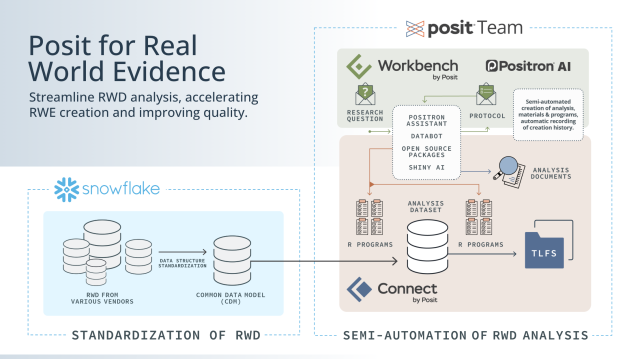
Posit and Snowflake together cover both ends of the RWE workflow: Snowflake as the governed data layer, Posit as the layer where analysis happens and gets shared, either running inside Snowflake’s own compute boundary or connecting into it from outside via OAuth — and, in either case, doing as much of the filtering and transformation as possible inside Snowflake itself before any data reaches local R or Python memory. What teams actually build on top of that combination — SAS-to-R bridging functions, shared analysis packages exposed through Shiny, AI-assisted (but human-reviewed) code generation, and CI/CD pipelines that make every study result traceable to a specific code version — looks a lot like ordinary software engineering practice applied to a domain (RWD/RWE) that has historically lacked it. The harder, still-unsolved parts of the pipeline — mapping heterogeneous RWD into CDISC SDTM, adjudicating line of therapy, harmonizing lab data across sources — aren’t solved by the stack itself; they’re where a lot of the real engineering and clinical judgment still has to happen, with tooling like this making that work faster and more auditable rather than automatic.
