Deploying boosted tree models with Orbital

Setting up

We’ll connect to a Snowflake database containing lending club loan data.

con <- DBI::dbConnect(
  odbc::snowflake(),
  warehouse = "DEFAULT_WH",
  database = "LENDING_CLUB",
  schema = "PUBLIC"
)

And load the packages that we need.

library(tidymodels)
library(orbital)
library(dbplyr)

── Attaching packages ────────────────────────────────────── tidymodels 1.4.1 ──

✔ broom        1.0.10     ✔ recipes      1.3.1 
✔ dials        1.4.2      ✔ rsample      1.3.1 
✔ dplyr        1.1.4      ✔ tailor       0.1.0 
✔ ggplot2      4.0.0      ✔ tidyr        1.3.1 
✔ infer        1.0.9      ✔ tune         2.0.0 
✔ modeldata    1.5.1      ✔ workflows    1.3.0 
✔ parsnip      1.4.1      ✔ workflowsets 1.1.1 
✔ purrr        1.1.0      ✔ yardstick    1.3.2 

── Conflicts ───────────────────────────────────────── tidymodels_conflicts() ──
✖ purrr::discard() masks scales::discard()
✖ dplyr::filter()  masks stats::filter()
✖ dplyr::lag()     masks stats::lag()
✖ recipes::step()  masks stats::step()

Getting the data ready

One of the nice things about working with dbplyr is that we can do our data wrangling lazily—the transformations get translated to SQL and run in the database. Here we’re parsing out the issue date and grabbing a sample of 2016 loans.

lendingclub_dat <- con |>
  tbl("LOAN_DATA") |>
  mutate(
    ISSUE_YEAR = as.integer(str_sub(ISSUE_D, start = 5)),
    ISSUE_MONTH = as.integer(
      case_match(
        str_sub(ISSUE_D, end = 3),
        "Jan" ~ 1, "Feb" ~ 2, "Mar" ~ 3, "Apr" ~ 4,
        "May" ~ 5, "Jun" ~ 6, "Jul" ~ 7, "Aug" ~ 8,
        "Sep" ~ 9, "Oct" ~ 10, "Nov" ~ 11, "Dec" ~ 12
      )
    )
  )

lendingclub_sample <- lendingclub_dat |>
  filter(ISSUE_YEAR == 2016) |>
  slice_sample(n = 5000)

lendingclub_prep <- lendingclub_sample |>
  select(INT_RATE, TERM, BC_UTIL, BC_OPEN_TO_BUY, ALL_UTIL) |>
  mutate(INT_RATE = as.numeric(str_remove(INT_RATE, "%"))) |>
  filter(!if_any(everything(), is.na)) |>
  collect()

Building a model the tidymodels way

Nothing special here—just a standard tidymodels workflow. We’re predicting the interest rate from a handful of credit utilization features using xgboost. Keep in mind that not all models or recipes steps are supported. See this vignette for a list of all supported methods.

lendingclub_rec <- recipe(INT_RATE ~ ., data = lendingclub_prep) |>
  step_dummy(TERM) |>
  step_normalize(all_numeric_predictors()) |>
  step_impute_mean(BC_OPEN_TO_BUY, BC_UTIL) |>
  step_filter(!if_any(everything(), is.na))

lendingclub_bt <- boost_tree(
  trees = tune(),
  tree_depth = tune(),
  learn_rate = tune()
) |>
  set_engine("xgboost") |>
  set_mode("regression")

lendingclub_wf <- workflow() |>
  add_model(lendingclub_bt) |>
  add_recipe(lendingclub_rec)

Tuning with SQL size in mind

When you’re deploying models to a database, SQL complexity matters. The number and depth of trees and how deep they are both influence how big the SQL expression for prediction will be. Too large expressions can hit database expression limits, or simply just take longer to evaluate than we would like.

orbital 0.5.1 introduces estimate_orbital_size(), which you can use as an extraction function during tuning. This lets you see how big the generated SQL will be for each model configuration.

Furthermore, we know that boosted trees generally have many different combinations of hyperparameters that yield similar predictive performance. Few trees with a large learning rate can perform just as well as many trees with a small learning rate.

Given that we want to keep our expression size as low as possible, we will modify the hyperparameter grid space to focus on smaller trees and fewer trees.

set.seed(1234)

grid <- extract_parameter_set_dials(lendingclub_wf) |>
  update(
    trees = trees(range = c(1, log10(500)), trans = transform_log10()),
    tree_depth = tree_depth(range = c(1, 7))
  ) |>
  grid_space_filling(size = 50)

bt_res <- tune_grid(
  lendingclub_wf,
  resamples = vfold_cv(lendingclub_prep),
  grid = grid,
  control = control_grid(
    extract = orbital::estimate_orbital_size
  )
)

Now we can visualize the tradeoff between predictive performance and SQL complexity:

size_tbl <- bt_res |>
  collect_extracts() |>
  summarise(avg_size = mean(unlist(.extracts)), .by = .config)

bt_res |>
  collect_metrics() |>
  left_join(size_tbl, by = ".config") |>
  filter(.metric == "rmse") |>
  ggplot(aes(x = avg_size, y = mean)) +
  geom_point() +
  labs(x = "SQL size (characters)", y = "RMSE") +
  scale_x_log10()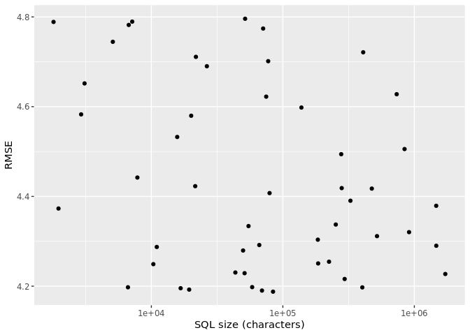

One of the striking revelations of this chart is that there is virtually no relationship between performance and SQL size. This should not be surprising because we know that there are multiple combinations of hyperparameters that yield good results.

Let us now pull out the top 5 combinations.

best_candidates <- show_best(bt_res, metric = "rmse") |>
  left_join(size_tbl, by = ".config") |>
  relocate(mean, std_err, avg_size)

best_candidates

# A tibble: 5 × 10
   mean std_err avg_size trees tree_depth learn_rate .metric .estimator     n
  <dbl>   <dbl>    <dbl> <int>      <int>      <dbl> <chr>   <chr>      <int>
1  4.19  0.0478   84222.   363          2     0.0149 rmse    standard      10
2  4.19  0.0478   69396    139          3     0.0483 rmse    standard      10
3  4.19  0.0476   19388.   207          1     0.0543 rmse    standard      10
4  4.20  0.0490   16697     33          3     0.250  rmse    standard      10
5  4.20  0.0476  402135.   393          4     0.0118 rmse    standard      10
# ℹ 1 more variable: .config <chr>

We see that they are all relatively close to each other. At least considering the standard error of the estimate. But what we see even more is that there is a big difference between the largest and smallest SQL estimates. With the largest expression being over 24 times that of the smallest.

Let us pick out the “best” performance values, as well as the biggest and smallest models.

param_best <- best_candidates |> slice_min(mean)
param_small <- best_candidates |> slice_min(avg_size)
param_large <- best_candidates |> slice_max(avg_size)

Does SQL size actually matter?

We’ve been talking about SQL complexity, but does it really affect performance? Let’s find out by comparing prediction times for models with different SQL sizes. We’ll fit two models: one with a small SQL footprint and one with a larger one.

# A model with the best RMSE
best_wf <- finalize_workflow(lendingclub_wf, param_best)
best_fit <- fit(best_wf, lendingclub_prep)
best_orb <- orbital(best_fit, separate_trees = TRUE)

# A model with smaller SQL (fewer/shallower trees)
small_wf <- finalize_workflow(lendingclub_wf, param_small)
small_fit <- fit(small_wf, lendingclub_prep)
small_orb <- orbital(small_fit, separate_trees = TRUE)

# A model with larger SQL (more/deeper trees)
large_wf <- finalize_workflow(lendingclub_wf, param_large)
large_fit <- fit(large_wf, lendingclub_prep)
large_orb <- orbital(large_fit, separate_trees = TRUE)

Now let’s time the predictions on the full dataset:

# Time the "best" model
best_time <- system.time({
  best_preds <- predict(best_orb, lendingclub_dat) |>
    compute(name = "LENDING_CLUB_PREDICTIONS_TEMP_BEST")
})

# Time the smaller model
small_time <- system.time({
  small_preds <- predict(small_orb, lendingclub_dat) |>
    compute(name = "LENDING_CLUB_PREDICTIONS_TEMP_SMALL")
})

# Time the larger model
large_time <- system.time({
  large_preds <- predict(large_orb, lendingclub_dat) |>
    compute(name = "LENDING_CLUB_PREDICTIONS_TEMP_LARGE")
})

tibble(
 model = c("Best SQL", "Small SQL", "Large SQL"),
 elapsed_seconds = c(best_time["elapsed"], small_time["elapsed"], large_time["elapsed"])
)

# A tibble: 3 × 2
  model     elapsed_seconds
  <chr>               <dbl>
1 Best SQL            48.0 
2 Small SQL            9.99
3 Large SQL          502.  

The difference can be substantial, especially as your data grows. This is why tracking SQL size during tuning is so valuable—you can make an informed choice about whether the extra predictive power is worth the computational cost.

Why are we using separate_trees?

Let’s see what happens when we try the default approach:

orb_combined <- orbital(best_fit, separate_trees = FALSE)

predict(orb_combined, lendingclub_dat) |>
  compute(name = "LENDING_CLUB_PREDICTIONS_TEMP_FALSE")

The prediction fails because Snowflake hits its expression depth limit. When separate_trees = FALSE, all trees are combined into a single massive expression, and databases have limits on how deeply nested expressions can be.

This is exactly why orbital 0.5.0 introduced the separate_trees argument. When set to TRUE, each tree is emitted as a separate intermediate column before being summed. This keeps individual expressions small enough and lets columnar databases like Snowflake evaluate trees in parallel.

Wrapping up

The workflow we’ve shown here, built in tidymodels, deploys with orbital, letting data scientists stay in their preferred tools while getting production-grade database performance. With the new SQL size tracking in orbital 0.5.0, you can make informed decisions about the accuracy-complexity tradeoff before deployment.

One thing to keep in mind: tree-based models like XGBoost use 32-bit floats internally, while R and databases typically use 64-bit precision. This can occasionally cause small prediction differences at split boundaries. See the floating-point precision vignette for details on when this matters and how to test for it.