Geospatial distributed processing with furrr


This is a guest post from Ryan Garnett, Data Management Insights & Analytics Manager at Green Shield Canada. Ryan works to bridge technical teams and senior executives by effectively communicating complex transformational change, achieved through international experience in technology development, operational management, client service, and strategic development. Keep in touch on LinkedIn.
The challenge
Everything happens somewhere. Location is an important factor when people make decisions that influences various life decisions, from buying a house, choosing a school, to vacations, or selecting a restaurant to eat out at. Within the data space utilizing location data is becoming increasingly important in data analysis, data science, and machine learning. Data wrangling is an integral part of data science, typically occupying a significant portion of time and effort, with location data adding to the complexity.
Location data can be large, consisting of hundreds of thousands to billions of observations in a single dataset. With location-based analysis consistently utilizing multiple datasets, the time to complete the analysis can be lengthy. Similar to other data analytics, the majority of location-based analysis tasks are performed sequentially using a single processor on a computer, even though many of the operations performed have no dependency on the other data or their outcome; if only there were another way…well, let me introduce you to distributed location-based processing.
What is distributed processing? In short, distributed processing is the use of multiple computer processors to execute a single computational task. A distributed process is executed by splitting a task into smaller chunks which are simultaneously performed on multiple processors. We can use distributed processing to make our code run faster, sometimes much faster. For large geospatial datasets that require a lot of computational power, distributed processing can reduce the time needed to handle complex data manipulation.
In this post, we’ll explore different techniques for wrangling location data, the processing time required for each, and the significant improvements that can be seen with distributed processing.
Setup
We performed the analysis for the post on a System76 Ubuntu laptop with the following configurations:
1 Operating System Ubuntu 22.04
2 Cores 8
3 CPU speed 1.80GHz
4 RAM 32GBLoad packages
We use a number of packages in this post, some standard data analytics packages ({dplyr}, {janitor}, {ggplot2}, {gt}, and {readr}), as well as a few niche packages ({furrr}, {future}, {leaflet}, and {sf}).
The goal of {furrr} is to combine {purrr}’s family of mapping functions with {future}’s parallel processing capabilities: {furrr} R package
The {future} package provides unified parallel and distributed processing in R for everyone: {future} R package
Leaflet is one of the most popular open-source JavaScript libraries for interactive maps: {leaflet} R package
The {sf} package provides access, data wrangling, and data analysis for location data: {sf} R package
# Importing data
library(readr)
# Data analysis and wrangling
library(dplyr)
library(janitor)
library(sf)
# Distributed processing
library(furrr)
library(future)
# Visualization and styling
library(ggplot2)
library(gt)
library(leaflet)Helper functions
We will use location data from different sources with different attribute standards. To assist with the data wrangling, we create custom functions to help standardize attributes available within the source datasets.
# Add provincial abbreviation column from provincial name
create_prov_abbrv_from_name <- function(.data, prov_column){
.data %>%
dplyr::mutate(PROV = dplyr::case_when(
{{prov_column}} == "Alberta" ~ "AB",
{{prov_column}} == "British Columbia" ~ "BC",
{{prov_column}} == "Manitoba" ~ "MB",
{{prov_column}} == "New Brunswick" ~ "NB",
{{prov_column}} == "Newfoundland and Labrador" ~ "NL",
{{prov_column}} == "Northwest Territories" ~ "NT",
{{prov_column}} == "Nova Scotia" ~ "NS",
{{prov_column}} == "Nunavut" ~ "NU",
{{prov_column}} == "Ontario" ~ "ON",
{{prov_column}} == "Prince Edward Island" ~ "PE",
{{prov_column}} == "Quebec" ~ "QC",
{{prov_column}} == "Saskatchewan" ~ "SK",
{{prov_column}} == "Undersea Feature" ~ "Non Province",
{{prov_column}} == "Yukon" ~ "YK",
TRUE ~ "Non Canadian"
))
}
# Add provincial abbreviation column from provincial id value
create_prov_abbrv_from_census_num <- function(.data, column_name){
.data %>%
dplyr::mutate(PROV = dplyr::case_when(
{{column_name}} == 10 ~ "NL",
{{column_name}} == 11 ~ "PE",
{{column_name}} == 12 ~ "NS",
{{column_name}} == 13 ~ "NB",
{{column_name}} == 24 ~ "QC",
{{column_name}} == 35 ~ "ON",
{{column_name}} == 46 ~ "MB",
{{column_name}} == 47 ~ "SK",
{{column_name}} == 48 ~ "AB",
{{column_name}} == 59 ~ "BC",
{{column_name}} == 60 ~ "YK",
{{column_name}} == 61 ~ "NT",
{{column_name}} == 62 ~ "NU",
TRUE ~ "Non Canadian"
))
}
# Change case of sf geometry column
change_sf_geometry_case <- function(df){
names(df)[names(df) == "geometry"] <- "GEOMETRY"
attr(df, "sf_column") <- "GEOMETRY"
df
}Source data
Location data, also known as geospatial data, is a specific type of data that stores geographic coordinates for use in analysis and visualizations. There are two main types of location data: vector and raster. This blog post will leverage vector data, which consists of points, lines, or polygons.
Points A unique location represented by X and Y locations, such as:
- address location
- place names
- points of interest (POI)
Lines A series of multiple point locations connected together in a linear path, such as:
- rivers
- roads
- trails
Polygons A set of enclosed connected points that represent a defined area, such as:
- countries
- land use
- water bodies
For this blog, we will use point and polygon vector data, specifically Canadian postal code (points) and Census Canada economic regions (polygons). For more information on the data sources, see the two links below.
# Open source Canadian postal codes
# Download, import, and transform data
can_postal_codes <-
readr::read_csv(
"https://raw.githubusercontent.com/ccnixon/postalcodes/master/CanadianPostalCodes.csv"
) %>%
janitor::clean_names("all_caps") %>%
create_prov_abbrv_from_census_num(FSA_PROVINCE) %>%
dplyr::select(FSA,
POSTAL_CODE,
PLACE_NAME,
PROV,
AREA_TYPE,
LATITUDE,
LONGITUDE) %>%
sf::st_as_sf(coords = c('LONGITUDE', 'LATITUDE'),
crs = 4326) %>%
sf::st_make_valid() %>%
change_sf_geometry_case()
# Statistics Canada economic regions data
# Download, import, and transform source zip file data
download.file(
"https://www12.statcan.gc.ca/census-recensement/2021/geo/sip-pis/boundary-limites/files-fichiers/ler_000b21a_e.zip",
destfile = "/data/ler_000b21a_e.zip"
)
# Unzip file
system("unzip /data/ler_000b21a_e.zip")
# Import and transform data
can_eco_regions <- sf::st_read("~/R/data/ler_000b21a_e.shp") %>%
janitor::clean_names("all_caps") %>%
create_prov_abbrv_from_census_num(PRUID) %>%
sf::st_transform(crs = 4326) %>%
sf::st_make_valid() %>%
dplyr::select(ERUID, ERNAME, PROV) %>%
change_sf_geometry_case()Data exploration
We will use two datasets for this analysis, Canadian postal code points and Canadian Census economic polygons. Both datasets have location information and have undergone data wrangling to standardize their attributes. Let’s take a quick look at the volume of each of the datasets.
| Dataset | Number of Columns | Number of Rows |
|---|---|---|
| Postal codes | 6 | 889,291 |
| Economic regions | 4 | 76 |
The postal code point dataset has the largest volume of data distributed across Canada. The following table outlines the number of postal code points in each province and territory.
| Province | Number of Points |
|---|---|
| AB | 86,977 |
| BC | 132,827 |
| MB | 27,833 |
| NB | 59,563 |
| NL | 11,344 |
| NS | 26,924 |
| NT | 604 |
| NU | 21 |
| ON | 295,166 |
| PE | 3,487 |
| QC | 218,745 |
| SK | 24,711 |
| YK | 1,089 |
While the volume of data in the polygon dataset is significantly smaller compared to the points layer, it should be noted that each polygon covers a large geographic area. The number of economic regions ranges from 1 to 17, depending on the province or territory.
| Province | Number of Polygons |
|---|---|
| AB | 8 |
| BC | 8 |
| MB | 8 |
| NB | 5 |
| NL | 4 |
| NS | 5 |
| NT | 1 |
| NU | 1 |
| ON | 11 |
| PE | 1 |
| QC | 17 |
| SK | 6 |
| YK | 1 |
The postal code points are not evenly distributed across the economic regions. Areas with larger populations and urban development have a greater number of postal codes, as illustrated on the map of Nova Scotia, where a high volume of points are positioned in two main areas.
Spatial intersection
A typical location data wrangling task is to pull attribute information from one location dataset based on the geographical position of another location dataset. To achieve this, we leverage the st_intersection() function from the sf package, allowing us to extract attribute information in the economic regions polygon to be added to the postal code point layer.
The approach of the st_intersection() function is to have each point “check” to see if it geographically intersects with a record in the polygon layer. This approach is challenging when you have large volumes of data that span a large geographic region, like the case in Canada. The standard approach with the st_intersection() function is to run the function with the whole point and polygon layers, which results in a lot of needless requests between the point and polygon layers (i.e., points in Nova Scotia checking if they geographically intersect with polygons in British Columbia). What if a common geographic area could separate the points and polygons, reducing the volume of the data and allowing for chunks to be processed simultaneously on different computer cores? In theory, this is a fast approach.
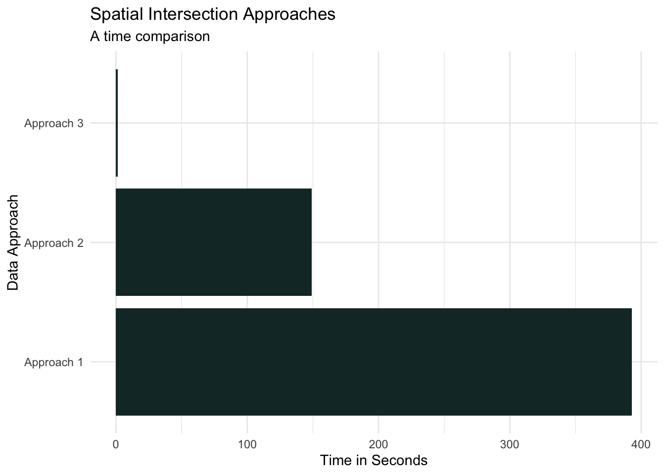
To test the theory, let’s select a sub-sample of the postal code point layer and run the st_intersection() function in three different approaches:
- All points and all polygons (the standard approach)
- Geographic region of points and all polygons (province of points and Canada-wide polygons)
- Geographic region of points with the same geographic region of polygons
can_postal_codes_sample <- can_postal_codes %>%
dplyr::sample_n(100000)
ns_sample_pnts <- nrow(as.data.frame(can_postal_codes_sample) %>%
dplyr::filter(PROV == "NS"))
# Approach 1
sf::st_intersection(can_postal_codes_sample,
dplyr::select(can_eco_regions, ERUID, ERNAME))
# Approach 2
sf::st_intersection(
dplyr::filter(can_postal_codes_sample, PROV == "NS"),
dplyr::select(can_eco_regions, ERUID, ERNAME)
)
# Approach 3
sf::st_intersection(
dplyr::filter(can_postal_codes_sample, PROV == "NS"),
dplyr::select(dplyr::filter(can_eco_regions, PROV == "NS"), ERUID, ERNAME)
)This test should help us understand if our theory of simultaneously processing chunks of data (aka distributed processing) reduces data wrangling time. Using the sample_n() function from {dplyr}, we randomly select 100,000 postal code points for use in Approach 1, and ns_sample_pnts() points being used in Approach 2 and Approach 3, which result in the following processing times:
- Approach 1 - The standard approach: The following are the volume of data used in this approach and the processing time.
| Point layer | 100,000 randomly selected points across Canada |
| Polygon layer | 76 polygons across Canada |
| Processing time | 6.6 minutes |
- Approach 2 - Province of points and Canada-wide polygons: The following are the volume of data used in this approach and the processing time.
| Point layer | 3,026 randomly selected points across Nova Scotia |
| Polygon layer | 76 polygons across Canada |
| Processing time | 2.5 minutes |
- Approach 3 - Province of points and polygons: The following are the volume of data used in this approach and the processing time.
| Point layer | 3,026 randomly selected point across Nova Scotia |
| Polygon layer | 5 polygons across Nova Scotia |
| Processing time | 1.2 seconds |
The results from the test validate the theory that processing points and polygons separated geographically is significantly faster than the alternative approaches.
Distributed processing with R
Now, let’s distributively process the Canada-wide postal codes with the Canada-wide economic regions.
There are several different options for distributed processing within R, but we will leverage the {future} and {furrr} packages for this story. One of the advantages of using {furrr} is that it follows the tidyverse syntax, with a few of {furrr}’s functions looking very similar to {purrr} functions. This approach provides ample power without the need to learn new programming languages, frameworks, or additional computer resources.
To take advantage of distributed processing, we need to prepare the data and select the distributed methods before performing the processing. To distribute process the Canada-wide postal codes and economic regions, we do the following four things:
- Break data into smaller chunks
- Split the postal code points by province
- Split the economic region polygon by province
- Identify the distributed method
- Run a multisession using eight cores
- Perform the processing
- Intersect points with polygons using the
st_intersection()function
- Intersect points with polygons using the
- Combine the results
- Bind the rows from each process into a single data frame
# Split Data by Province
# Postal codes -- points
can_pcodes_split <- can_postal_codes %>%
dplyr::filter(PROV != "Non Canadian") %>%
dplyr::group_by(PROV) %>%
dplyr::group_split()
# Economic regions -- polygons
can_eco_regions_split <- can_eco_regions %>%
dplyr::group_by(PROV) %>%
dplyr::group_split()
# Distribute the processing
future::plan(multisession, workers = 8)
furrr::future_map2(can_pcodes_split, can_eco_regions_split, sf::st_intersection) %>%
dplyr::bind_rows()- Distributed processing - Canada-wide points and polygons The following are the volume of data used in this approach and the processing time.
| Point layer | 889,291 point across Canada |
| Polygon layer | 76 polygons across Canada |
| Processing time | 3.6 minutes |
Our findings
The results from the analysis were eye-opening. Breaking the data into smaller chunks allowed us to process our data simultaneously, significantly decreasing processing time. The Canada-wide distributed processing was completed in 3.6 minutes, almost two times faster than the 100,000 randomly sampled postal code points processed using traditional methods. Using the sample processing time to estimate Canada-wide, non-distributed processing time results in 58.3 minutes, which would be 16x longer than the distributed processing time!
Summary
Data wrangling is an unavoidable part of any data project, occupying a significant portion of time and resources. Reducing the effort during this stage allows more time to be allocated during analysis and modelling. Distributed processing is an option that can be implemented in certain data-wrangling situations that can seriously reduce processing time, not just in geospatial applications but in non-location data as well. With most, if not all, new computers being equipped with multiple processors, distributed processing becomes a low-cost solution that many data teams can employ to improve their data science pipelines.

Ryan Garnett
Related Content

What makes Posit different from proprietary analytics vendors

Deploying boosted tree models with Orbital
