Tiny Doses for Tiny Babies -- How much is too much?

If you have fit a mixed model, you have done half of this

Drug exposure is a dynamic process. As a drug is being absorbed, it is also being distributed throughout the body, and cleared at the same time. Pharmacometric (PMX) models help us to address these dynamic processes acting together via ordinary differential equations (ODE). Think like a filling a bucket of water with a hole at the bottom - how fast the bucket fills depends on how fast the rate of water flows in vs flows out.

In pharmacometrics we understand, like other fields, we have different infant sizes, and different ways the drug flows, which means a method to solve differential equations, and characterize differences between individuals at the same time: the mean function inside the nonlinear mixed model that is not a line or a spline, it is the solution to a system of ODEs describing how drug moves through the body.

These movements and concentrations are characterized by two parameters the clearance (volume of blood eliminated of drug per hour) and volume of distribution (how widely the drug spreads through tissue), you can use these are physiological quantities to inform the mechanism of how the drug works. In the field the movement of concentrtaions in the model is called a pharmacokinetic (PK) model.

PK models are great because they:

• They extrapolate. Once you know clearance, you know the concentration for a dose nobody in your study ever received.
• They can describe meaningful relationships. Clearance scales with body size and kidney function; volume scales with body water. This has been studied by the field in models for quite awhile. Therefore, when you are using population level ways of better describing the data (ie covariates), you put them on where biology says they belong, not where it simply better describe the data.
• They separate the parts of a regimen. The loading dose is governed by volume; the maintenance dose is governed by clearance. Estimating them separately is exactly what lets you design a regimen, and it is invisible if all you have is a fitted curve.

So the questions pharmacometrics answers are dosing questions: what dose, how often, by what route; who needs a different one (children, renal impairment, drug interactions, obesity etc); what happens when a dose is missed; how much exposure produces the effect and how much starts producing harm; and whether the Phase III trial is worth running at all, at which dose.

Dosing sections of drug labels are built from these models. Pediatric doses are routinely approved by adult model extrapolation rather than and unjustified pediatric trial.

In the clinic, these models help therapeutic drug monitoring – vancomycin (for MRSA infections), busulfan (for cancer), infliximab (Autoimmune/inflamitory) – where the need of the drug is great and individual variability of effect / toxicity needs to be carefully balanced in each individual. Both FDA and EMA have written guidance on population pharmacokinetics. It is a small field with an unusually direct path from a model object to what happens to a patient.

The data

In this example we are using this dataset: 59 preterm infants given phenobarbital, published by Grasela and Donn in 1985. It ships with nlmixr2 as pheno_sd.

library(nlmixr2)
head(pheno_sd, 4)

##   ID TIME  AMT  WT APGR   DV MDV EVID
## 1  1  0.0 25.0 1.4    7  0.0   1    1
## 2  1  2.0  0.0 1.4    7 17.3   0    0
## 3  1 12.5  3.5 1.4    7  0.0   1    1
## 4  1 24.5  3.5 1.4    7  0.0   1    1

The columns are the pharmacometric standard: ID, TIME, AMT (amount or dose given), DV (dependent variable, in this case concentration), EVID (1 = dose, 0 = observation) plus covariates WT (kg) and APGR (Apgar score). The nlmixr2 format is very similar to the NONMEM format since it is prevalent across the field.

One of the first things to do is do some exploration of the data:

obs <- subset(pheno_sd, EVID == 0)

c(infants       = length(unique(pheno_sd$ID)),
  doses         = sum(pheno_sd$EVID == 1),
  concentrations = nrow(obs))

##        infants          doses concentrations
##             59            589            155

table(`samples per infant` = table(obs$ID))

## samples per infant
##  1  2  3  4  5  6
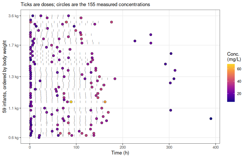
##  9 15 27  6  1  1

Nine infants have exactly one concentration. Forty percent have two or fewer. There are 589 doses and only 155 measurements — the infants were dosed relentlessly and sampled infrequently during routine care.

You can see this clearly with the following exploratory plot:

Step 1: A first nlmixr2 model

First, we need to build a PK model. To describe the model you can use an ordinary R function with two blocks – an ini({}) and a model({}) block:

pheno <- function() {
  ini({
    tcl <- log(0.008)   # log typical clearance (L/h)
    tv  <- log(0.6)     # log typical volume (L)
    eta.cl ~ 1          # between-infant variability on clearance
    eta.v  ~ 1          # between-infant variability on volume
    prop.sd <- 0.1      # proportional residual error
  })
  model({
    cl <- exp(tcl + eta.cl)
    v  <- exp(tv  + eta.v)
    d/dt(central) <- -(cl / v) * central
    cp <- central / v
    cp ~ prop(prop.sd)
  })
}

Three things are worth pointing out, because they are the whole language:

• ini({}) holds initial estimates. <- declares a fixed effect (and residual estimates) ~ declares a random effect with its initial variance.
• model({}) is the model itself. d/dt(central) is a differential equation, declared in Lebneitz notation. This one says drug leaves the central compartment at a rate proportional to how much is there. Dosing is driven by the data (AMT/EVID), so doesn’t appears in this model code.
• The last line, cp ~ prop(prop.sd), says the observed concentration is the predicted cp with proportional residual error. That is where the model meets dependent variable, DV.

Everything else is plain R. WT will be a column in the data; exp() is exp().

Fitting it:

# note here we use the := nlmixr2 save function to cache the fit
# since nonlinear mixed effects models can take some time to run.
fit1 := nlmixr2(pheno, pheno_sd, est = "saem",
                control = saemControl(print = 0, seed = 42),
                table = tableControl(cwres = TRUE, npde = TRUE))

You can print out the entire fit object, which is a modified data-frame of predictions and estimates together. Another way to look at the data is simply to look at the estimate:

fit1$parFixedDf[, c("Estimate", "Back-transformed", "BSV(CV%)")]

##           Estimate Back-transformed BSV(CV%)
## tcl     -5.1900879      0.005571517 38.93382
## tv       0.3523780      1.422446081 46.69663
## prop.sd  0.1248964      0.124896392       NA

Typical clearance is about r signif(exp(fit1$parFixedDf["tcl","Estimate"]), 3) L/h and typical volume about 1.42 L. But look at the last column: between-infant variability of 37% on clearance and 47% on volume. Two infants drawn at random from this population can easily differ two-fold in exposure on the same dose. That is the number that makes a single flat dose dangerous, and the next question is whether any of it is explainable.

One line, and half the variability disappears

These infants weigh between 0.6 and 3.6 kg – a six-fold range in body size. It would be strange if that did not matter. Larger bodies have larger livers and kidneys and more water to distribute drug into, and the standard way to encode that is allometric scaling: clearance scales with weight to the 3/4 power, volume scales linearly.

In general this covariate, and others, are there to explain why certain babies/individuals have more drug in their system than others.

The change to the model is one line each. In nlmixr2 instead of having to rewrite the whole model we can change pieces of the model with model piping:

phenoWt <-  pheno |>
  # first we modify the cl line
  model(cl <- exp(tcl + eta.cl + cov.cl.wt*log(WT/1.3))) |>
  # then the v line
  model(v  <- exp(tv  + eta.v  + cov.v.wt*log(WT/1.3))) |>
  # then we add the covariate effects to the ini block
  ini(cov.cl.wt=0.75, cov.v.wt=1)

fit2 := nlmixr2(phenoWt, pheno_sd, est = "saem",
                control = saemControl(print = 0, seed = 42),
                table = tableControl(cwres = TRUE, npde = TRUE))

tibble(
  model = c("Base", "+ allometric weight"),
  OBJF  = c(fit1$objf, fit2$objf),
  AIC   = c(AIC(fit1), AIC(fit2)),
  `BSV CL (CV%)` = c(fit1$parFixedDf["tcl", "BSV(CV%)"],
                     fit2$parFixedDf["tcl", "BSV(CV%)"]),
  `BSV V (CV%)`  = c(fit1$parFixedDf["tv", "BSV(CV%)"],
                     fit2$parFixedDf["tv", "BSV(CV%)"])
) %>% mutate(across(where(is.numeric), ~ signif(.x, 4)))

## # A tibble: 2 × 5
##   model                OBJF   AIC `BSV CL (CV%)` `BSV V (CV%)`
##   <chr>               <dbl> <dbl>          <dbl>         <dbl>
## 1 Base                 736. 1030            38.9          46.7
## 2 + allometric weight  592.  890.           19.0          17.7

The objective function drops by about 144 points for two estimated parameters. Between-infant variability falls from 37% to 17% on clearance and from 47% to 18% on volume. This means more than half of the variability in these infants is just body weight which is why the infants are dosed by weight.

Leaning into the AI estimation methods

Experimentally, as of nlmixr2 7.0, we also allow variable-auto-encoding method (vae) to automatically select covariates with the l0learn method from google labs. These new nonlinear mixed effects routines lean into the new advancements in AI and apply them to this space. Using this method we get:

fit3 := nlmixr2(pheno, pheno_sd, est = "vae",
                control=vaeControl(print=0),
                table = tableControl(cwres = TRUE, npde = TRUE))

## calculating covariance matrix

This shows a full covariate search would have picked weight throughout as a covariate. You can see the full model with the covariates filled in here:

print(fit3$ui)

##  ── rxode2-based free-form 1-cmt ODE model ──────────────────────────────────────
##  ── Initalization: ──
## Fixed Effects ($theta):
##                   tcl                    tv               prop.sd
##            -5.1232496             0.2728871             0.1405524
##     beta.tcl.WT.power beta.tv.WT.hockey.low  beta.tv.WT.hockey.hi
##             0.6336053             0.9486716             0.5203213
##
## Omega ($omega):
##            eta.cl      eta.v
## eta.cl 0.02550034 0.00000000
## eta.v  0.00000000 0.01905948
##
## States ($state or $stateDf):
##   Compartment Number Compartment Name
## 1                  1          central
##  ── μ-referencing ($muRefTable): ──
##   theta    eta level
## 1   tcl eta.cl    id
## 2    tv  eta.v    id
##                                                                                        covariates
## 1                                                   log(0.769230769230769 * WT)*beta.tcl.WT.power
## 2 (-1.3 + WT) * (WT >= 1.3)*beta.tv.WT.hockey.hi + (WT < 1.3) * (-1.3 + WT)*beta.tv.WT.hockey.low
##
##  ── Model (Normalized Syntax): ──
## function() {
##     ini({
##         tcl <- -5.12324963707
##         tv <- 0.272887052962
##         prop.sd <- c(0, 0.140552353242)
##         beta.tcl.WT.power <- 0.63360525514
##         beta.tv.WT.hockey.low <- 0.948671628394
##         beta.tv.WT.hockey.hi <- 0.520321310437
##         eta.cl ~ 0.0255003432707
##         eta.v ~ 0.0190594819482
##     })
##     model({
##         cl <- exp(tcl + beta.tcl.WT.power * log(WT/1.3) + eta.cl)
##         v <- exp(tv + beta.tv.WT.hockey.low * (WT < 1.3) * (WT -
##             1.3) + beta.tv.WT.hockey.hi * (WT >= 1.3) * (WT -
##             1.3) + eta.v)
##         d/dt(central) <- -(cl/v) * central
##         cp <- central/v
##         cp ~ prop(prop.sd)
##     })
## }

And the same comparison for these weight covariates are here:

tibble(
  model = c("Base", "+ allometric weight"),
  OBJF  = c(fit1$objf, fit3$objf),
  AIC   = c(AIC(fit1), AIC(fit3)),
  `BSV CL (CV%)` = c(fit1$parFixedDf["tcl", "BSV(CV%)"],
                     fit3$parFixedDf["tcl", "BSV(CV%)"]),
  `BSV V (CV%)`  = c(fit1$parFixedDf["tv", "BSV(CV%)"],
                     fit3$parFixedDf["tv", "BSV(CV%)"])
) %>% mutate(across(where(is.numeric), ~ signif(.x, 4)))

## # A tibble: 2 × 5
##   model                OBJF   AIC `BSV CL (CV%)` `BSV V (CV%)`
##   <chr>               <dbl> <dbl>          <dbl>         <dbl>
## 1 Base                 736. 1030            38.9          46.7
## 2 + allometric weight  613.  914.           16.1          13.9

Further reducing the variability in volume to 14%

Does the model deserve to be believed?

First, individual profiles. This is where the borrowing of strength becomes visible:

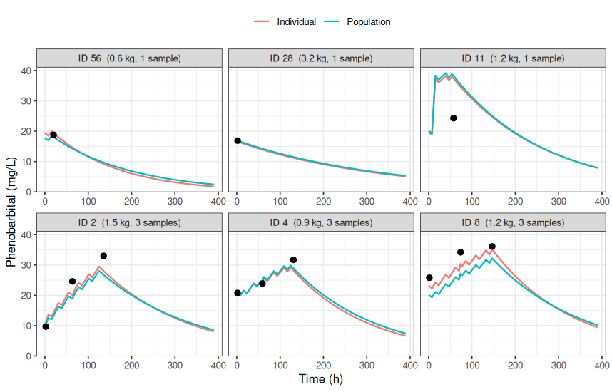
Infants 56 and 28 contributed one measurement each, and both come out with a complete concentration-time profile. The individual (red) and population (blue) curves nearly coincide – with one data point there is nothing to move the individual away from the population, which is exactly the right behavior. For infants 2 and 8, with three samples each, the two curves separate: there is now enough information to say this infant is not typical.

Second, a prediction-corrected visual predictive check — simulate many replicates of the study from the fitted model and ask whether the real data looks like a plausible draw:

vpcPlot(fit3, n = 300, pred_corr = TRUE, show = list(obs_dv = TRUE)) +
  labs(x = "Time (h)", y = "Prediction-corrected phenobarbital (mg/L)") +
  theme_bw()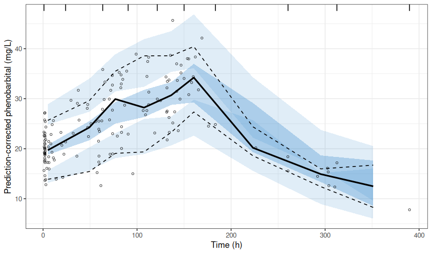

The observed median and 5th/95th percentiles (solid and dashed lines) sit inside the simulated bands across the study. With 155 observations the percentiles are noisy but it is not misspecified.

Step 2: Answering the actual question

Since we have captured the relationship of weight and CL, we can run the simulation of both weight based and flat dosing to see if both regimens are similar. The therapeutic target is roughly 15-40 mg/L.

Two candidates. A flat regimen — one dose for every infant, chosen to be correct for the average 1.5 kg baby in this study. And a weight-based regimen in mg/kg. Both use a loading dose (which volume of distribution determines) followed by twice-daily maintenance (which clearance determines).

The simulation reuses the fitted object directly — rxSolve() takes fit3 and samples new infants from its estimated between-subject distribution:

set.seed(99)
wts <- seq(0.7, 3.5, by = 0.2)

simOne <- function(w, reg) {
  flat <- grepl("^Flat", reg)
  ev <- et(amt = if (flat) 30  else 20   * w) %>%                # loading
        et(amt = if (flat) 1.9 else 1.25 * w,                    # maintenance
           ii = 12, until = 24 * 14, time = 12) %>%
        et(seq(24 * 7, 24 * 14, by = 4))                         # sample week 2
  rxSolve(fit3, ev, nSub = 400, iCov = data.frame(WT = w),
          addDosing = FALSE) %>%
    as.data.frame() %>% mutate(WT = w, regimen = reg)
}

grid <- expand.grid(
  WT = wts,
  regimen = c("Flat: 30 mg load + 1.9 mg q12h",
              "Weight-based: 20 mg/kg load + 1.25 mg/kg q12h"),
  stringsAsFactors = FALSE)

sim <- bind_rows(Map(simOne, grid$WT, grid$regimen))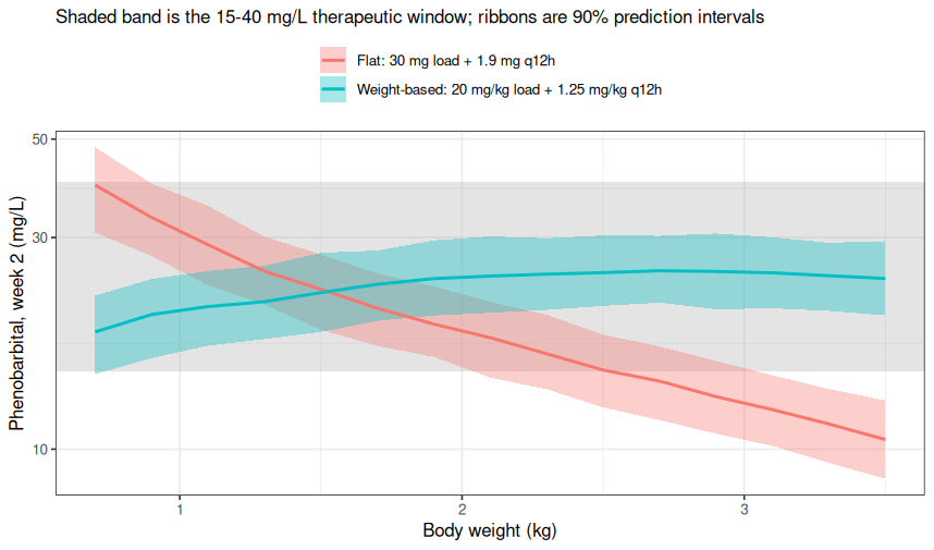

sim %>%
  filter(round(WT, 1) %in% c(0.7, 1.5, 2.3, 3.1)) %>%
  group_by(regimen, WT) %>%
  summarise(median = median(cp),
            `% in window` = 100 * mean(cp >= 15 & cp <= 40),
            .groups = "drop") %>%
  mutate(across(where(is.numeric), ~ round(.x, 1))) %>%
  arrange(regimen, WT)

## # A tibble: 8 × 4
##   regimen                                          WT median `% in window`
##   <chr>                                         <dbl>  <dbl>         <dbl>
## 1 Flat: 30 mg load + 1.9 mg q12h                  0.7   39.4          55.5
## 2 Flat: 30 mg load + 1.9 mg q12h                  1.5   22.9         100
## 3 Flat: 30 mg load + 1.9 mg q12h                  2.3   16.4          78.1
## 4 Flat: 30 mg load + 1.9 mg q12h                  3.1   12.3           3.3
## 5 Weight-based: 20 mg/kg load + 1.25 mg/kg q12h   0.7   18.4          93.8
## 6 Weight-based: 20 mg/kg load + 1.25 mg/kg q12h   1.5   22.5         100
## 7 Weight-based: 20 mg/kg load + 1.25 mg/kg q12h   2.3   24.8         100
## 8 Weight-based: 20 mg/kg load + 1.25 mg/kg q12h   3.1   25           100

The flat regimen was chosen to be right for the average infant, and it is: at 1.5 kg the median lands at 23 mg/L, comfortably mid-window, with every simulated infant in range. But it fails at both ends. The median 0.7 kg infant sits at 39 mg/L – pressed against the top of the window, with only about half of infants inside it – while at 3.1 kg the median has fallen to 12 mg/L and fewer than 4% of infants reach a therapeutic concentration at all. That is a more than three-fold exposure gradient across the population, driven entirely by a covariate that was sitting in the dataset the whole time.

The weight-based regimen holds the median between 19 and 25 mg/L across the entire weight range, with 96% or more of simulated infants inside the window at every weight.

There is a subtlety worth noticing in that curve: the weight-based line still drifts gently upward with weight then plateaus.

A caveat, stated clearly: this is a teaching example on a 1985 dataset, deliberately kept to one compartment and one covariate. It is not dosing guidance. Real neonatal phenobarbital dosing accounts for postnatal age and maturation, and would be under the care of a qualified doctor and pharmacist. The workflow, though, is the real one.

Where this sits in the R ecosystem

The part that is easy to miss in a walkthrough is that nothing above required leaving R. Many tools in pharmacometrics require a shuttle back and forth between 2 different tools and ecosystems.

The fit object is a modified tibble. as.data.frame(fit2) gives you observations, predictions, residuals, and empirical Bayes estimates in a tidy frame, which is why every plot in this post is plain ggplot2 and every summary is plain dplyr. There is no export step, no intermediate file format, no separate post-processing tool with its own data conventions. That sounds like a convenience and is really a reproducibility property: the places where analyses usually become irreproducible are the boundaries between tools, and this workflow does not have any.

That matters concretely. The whole thing — data prep, fit, diagnostics, simulation, report — is one Quarto or R Markdown document (this post is one).

One approach to keep this reproducible is to in the dependencies with renv, wire the fits into a targets pipeline so they only re-run when the model changes, and someone else can reproduce the dosing recommendation from the raw data with the R script or report.

The second thing worth knowing is that nlmixr2 is not a walled garden, which is unusual for this field and is probably the strongest practical argument for adopting it:

• babelmixr2 takes the same model object you just read and runs it through NONMEM or Monolix. You are not choosing a camp — you can fit in nlmixr2 and confirm in NONMEM, which is a genuinely useful thing to be able to do when the model matters. It also connects to PKNCA for non-compartmental initial estimates and PopED for optimal design.
• nonmem2rx and monolix2rx go the other direction, importing finished NONMEM and Monolix runs into R so that a decade of legacy models can be simulated, plotted, and checked with the same tooling.
• rxode2 is the ODE solver underneath both fitting and simulation. The model used for the regimen comparison above is bit-for-bit the model that was fit — not a hand-re-implementation of it in a separate simulation tool, which is a classic source of quiet errors.
• The surrounding ecosystem — xpose.nlmixr2 and ggPMX for standardized diagnostics, tidyvpc for VPCs, shinyMixR for run management, nlmixr2rpt for Word and PowerPoint reports — is described in more detail in an earlier post.

And then the ordinary open-source argument, which lands harder in pharma than people outside it expect: there is no license to negotiate. An academic collaborator, a CRO, a reviewer, or a curious statistician two floors away can run your analysis today.

Getting started

If you are a pharmacometrician who has been meaning to try this, the first model is a smaller step than it looks — everything above is about forty lines of code.

install.packages("nlmixr2")

That brings in the estimation engine, the ODE solver, and the plotting and diagnostic packages. On Windows you will also want Rtools, since models are compiled to C for speed. Then:

library(nlmixr2)
fit <- nlmixr2(pheno, pheno_sd, est = "saem",
               control = saemControl(print = 0))

Some places to go next:

• The nlmixr2 website has the full model language reference and a gallery of worked examples.
• nlmixr2lib is a library of starting models, so a two-compartment model with transit absorption is a lookup rather than a derivation.
• If you are coming from NONMEM, nonmem2rx will translate a model you already trust, which is a considerably more comfortable way in than starting from a blank file.
• nlmixr2 7.0, released this month, made focei solve in parallel across all OpenMP-enabled platforms, so the fits in this post are quicker than they would have been a year ago.

And if you are coming from outside the field entirely — from sports analytics, from supply chain, from anywhere people fit hierarchical models to messy observational data – the thing worth taking away is the shape of the problem. Fifty-nine subjects, most with one or two observations, a mechanistic model with parameters that mean something, and a decision at the end that someone has to make on Tuesday whether or not the analysis is finished.

The phenobarbital data is from Grasela TH Jr and Donn SM, “Neonatal population pharmacokinetics of phenobarbital derived from routine clinical data,” Dev Pharmacol Ther. 1985;8(6):374-383.