Teaching chat apps about R packages


Imagine I open up an LLM-based chat app like claude.ai and ask the following:
How does .by work in dplyr?
In this example, Claude might then respond:
In dplyr (version 1.1.0+), .by is an argument that provides grouping for a single operation without changing the data structure. It works as a more convenient alternative to group_by() followed by ungroup().
Claude “knows” this because dplyr 1.1.0 was released in early 2023; by the time the LLM was trained in late 2024, there was a ton of information about it on the internet. How can I make a chat app that knows about the internal R package that my team is working on?
We’ve been hearing about this need from many folks, and have developed several tools to help data scientists tackle this problem quickly. In this post, I’ll outline the process of building chat apps with R that know about your use case.
The context window
The name of the game here is context: what information does the model need to have access to in order to answer your users’ questions effectively?
You can think of the context window as the model’s short-term memory. As an example, Claude 3.7 Sonnet has a context window of 200,000 tokens. What does this mean? If we go back to my initial request, I started off the chat with the question, “How does .by work in dplyr?” Loosely, a token is a word, so I’ve used up something like 6 of the 200,000 tokens that are available in Claude’s context window. Claude responded with a couple sentences—maybe 50 additional tokens. Imagine I then respond in this same chat session with the following:
Got it. Could you transition this code to use .by?
mtcars %>% group_by(cyl) %>% summarize(mean = mean(mpg))This message is around 30 tokens. Since I hadn’t moved to a new chat session, though, the context window up to this point contains my first “How does .by work in dplyr?”, the model’s response, and my new message: altogether, something like 86 tokens. There are two main points here:
So far in this conversation, I’ve used only a tiny, tiny fraction of the context window that’s available with Claude. Models can fit a lot of information in their “short-term memory.”
If you think about chat conversations where you go back and forth with a model, say, fifty times, that’s quite a few tokens. If I had to read that many words to get up to speed on a conversation, it’d take me several minutes. Likely, though, you can’t even tell the difference between how fast the model responds to your first message versus your fiftieth. Models “read” really fast.
The fact that these models are able to read a couple hundred thousand words in an instant and keep all of it in their “short-term memory” gives us the solution to our problem. We can describe how our package (or set of packages) works super thoroughly and allow the model to sift through all that information to find what it needs.
I’ll highlight two approaches to providing models with context: the system prompt and tool calls. The system prompt contains information that the model will always have access to, and tool calls allow the model to “fetch” additional information as it needs it before responding to the user. For some use cases, like assistants for very small packages, you can get away with only providing a system prompt. For others, like larger packages (or sets of packages), you’ll likely want to provide context with both a system prompt and tool calls.
Note
I’m focusing on using the system prompt and tool calls to teach models specifically about R packages, though it’s worth noting that these two approaches can be used to teach a model about anything, like a database or some policy document.
Tools of the trade
Before I describe those two approaches in detail, let’s quickly call out the R packages that make this possible. You’ll need the dev versions of each; install them with pak::pak(c("tidyverse/ellmer", "posit-dev/shinychat", "posit-dev/btw")). One-by-one:


ellmer makes it easy to use large language models (LLM) from R. It supports a wide variety of model providers, like Anthropic (Claude), OpenAI, local models hosted with ollama, and providers with security-oriented deployments like Azure OpenAI, AWS Bedrock, etc.
shinychat allows you to easily integrate ellmer chats into shiny chat apps. Apps built with shinychat will feel intuitive to users of chat apps like ChatGPT or claude.ai, integrating familiar UI elements for tool calling, error handling, etc.
btw makes it easy to describe stuff to LLMs. The package allows you to quickly collect plain text context on R package documentation, data frames, and file contents. (We’re still sanding off btw’s rough edges, so the package isn’t yet on CRAN.)
Loading each of those:
library(ellmer)
library(shinychat)
library(btw)
As an example ellmer chat, I’ll start a conversation with Claude 3.5 Sonnet:
client <- chat_anthropic()
client$chat("Tell me a joke about data scientists.")
#> What do you call a data scientist who's also a DJ?
#>
#> Someone who drops sick beats... and then performs time series analysis on them!Hm…🤔
ellmer chats like the one above can be passed directly to shinychat to launch a chat app in your browser:
chat_app(client)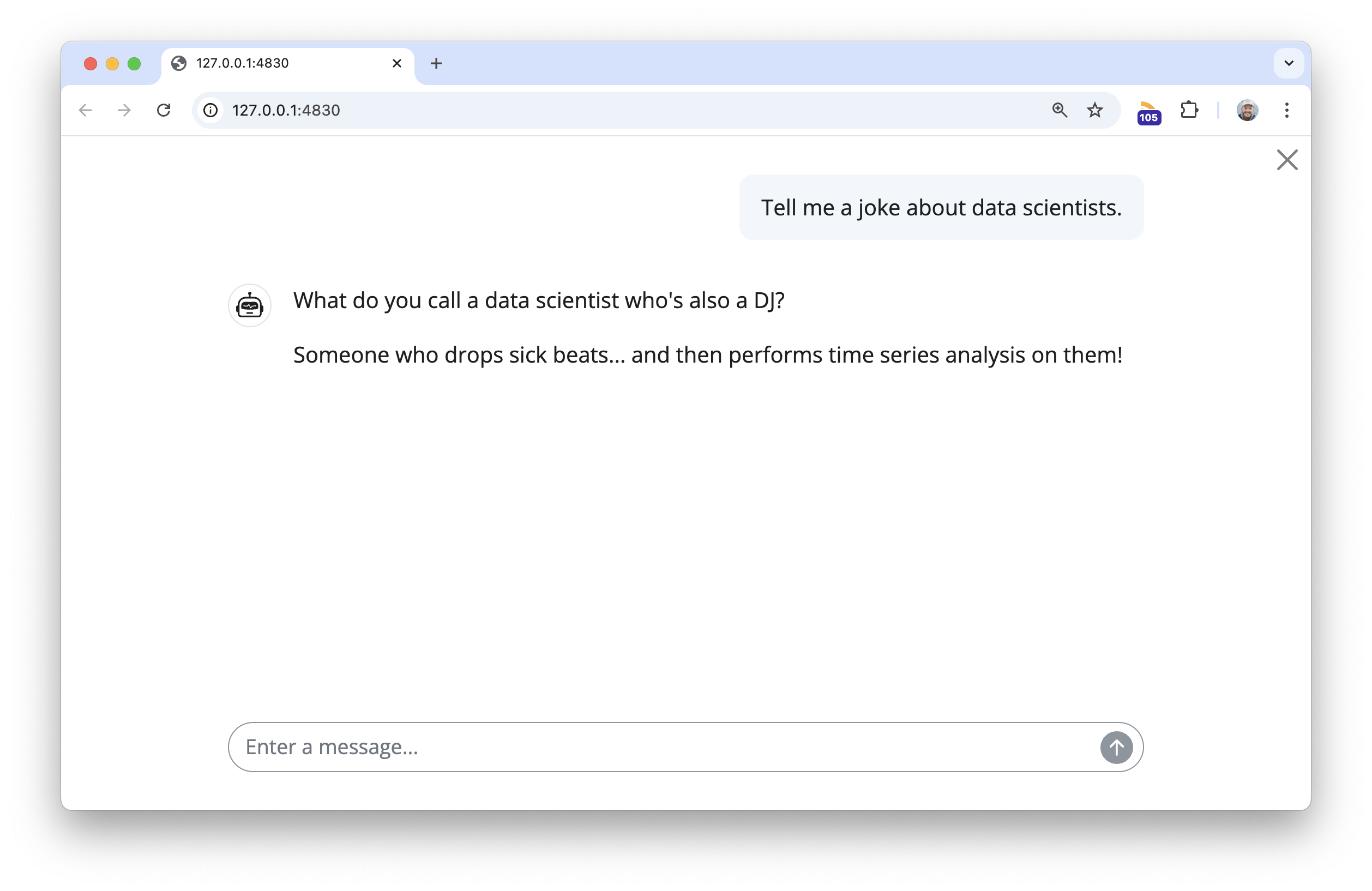
At this point, client is just a chat with the usual Claude 3.5 Sonnet model, no additional prompting or tools provided.
Static context: the system prompt
Imagine you could add an “invisible” message to the beginning of every chat. In that message, you could let the model know the kinds of questions it will be asked, how it should respond, and, importantly, things it should “know.” This is the system prompt.
When you think of what should live in the system prompt, try to answer this question: What will the model need to know about in almost every session it’s used in? When building chat apps for packages, you might consider including 1) The list of functions and help topics in the package documentation, 2) the introductory vignette, and, if needed, 3) the full documentation for a couple of the most important functions in your package.
The btw package provides shorthand for you to quickly compile this context from R. Revisiting our dplyr example, imagine I want to create a dplyr assistant. I could use this btw code to describe dplyr:
btw(
  # strings will be included as-is in the output, with the exception of
  # a few shorthand formats
  "You are a helpful but terse dplyr assistant.",
  # provide the full function reference and (if available) introductory vignette
  "{dplyr}",
  # include the full help-pages for filter(), mutate(), and summarize()
  ?dplyr::filter,
  ?dplyr::mutate,
  ?dplyr::summarize
)
✔ btw copied to the clipboard!btw() will copy the output to the clipboard, which you can paste directly into your system prompt. Especially for longer system prompts, it’s good practice to keep the system prompt in a persistent text file; across many frameworks, this file is called llms.txt. Here’s what the output from the above code looks like:
llms.txt for dplyr
You are a helpful but terse dplyr assistant.
## Context
"{dplyr}"
# Introduction to dplyr {#introduction-to-dplyr .title .toc-ignore}
When working with data you must:
- Figure out what you want to do.
- Describe those tasks in the form of a computer program.
- Execute the program.
The dplyr package makes these steps fast and easy:
- By constraining your options, it helps you think about your data
manipulation challenges.
- It provides simple "verbs", functions that correspond to the most
common data manipulation tasks, to help you translate your thoughts
into code.
- It uses efficient backends, so you spend less time waiting for the
computer.
This document introduces you to dplyr's basic set of tools, and shows
you how to apply them to data frames. dplyr also supports databases via
the dbplyr package, once you've installed, read `vignette("dbplyr")` to
learn more.
:::: {#data-starwars .section .level2}
## Data: starwars
To explore the basic data manipulation verbs of dplyr, we'll use the
dataset `starwars`. This dataset contains 87 characters and comes from
the [Star Wars API](https://swapi.dev), and is documented in `?starwars`
::: {#cb1 .sourceCode}
```{.sourceCode .r}
dim(starwars)
#> [1] 87 14
starwars
#> # A tibble: 87 × 14
#> name height mass hair_color skin_color eye_color birth_year sex gender
#> <chr> <int> <dbl> <chr> <chr> <chr> <dbl> <chr> <chr>
#> 1 Luke Sky… 172 77 blond fair blue 19 male mascu…
#> 2 C-3PO 167 75 <NA> gold yellow 112 none mascu…
#> 3 R2-D2 96 32 <NA> white, bl… red 33 none mascu…
#> 4 Darth Va… 202 136 none white yellow 41.9 male mascu…
#> # ℹ 83 more rows
#> # ℹ 5 more variables: homeworld <chr>, species <chr>, films <list>,
#> # vehicles <list>, starships <list>
```
:::
Note that `starwars` is a tibble, a modern reimagining of the data
frame. It's particularly useful for large datasets because it only
prints the first few rows. You can learn more about tibbles at
<https://tibble.tidyverse.org>; in particular you can convert data
frames to tibbles with `as_tibble()`.
::::
::::::::::::::::::::::::::::: {#single-table-verbs .section .level2}
## Single table verbs
dplyr aims to provide a function for each basic verb of data
manipulation. These verbs can be organised into three categories based
on the component of the dataset that they work with:
- Rows:
- `filter()` chooses rows based on column values.
- `slice()` chooses rows based on location.
- `arrange()` changes the order of the rows.
- Columns:
- `select()` changes whether or not a column is included.
- `rename()` changes the name of columns.
- `mutate()` changes the values of columns and creates new
columns.
- `relocate()` changes the order of the columns.
- Groups of rows:
- `summarise()` collapses a group into a single row.
::: {#the-pipe .section .level3}
### The pipe
All of the dplyr functions take a data frame (or tibble) as the first
argument. Rather than forcing the user to either save intermediate
objects or nest functions, dplyr provides the `%>%` operator from
magrittr. `x %>% f(y)` turns into `f(x, y)` so the result from one step
is then "piped" into the next step. You can use the pipe to rewrite
multiple operations that you can read left-to-right, top-to-bottom
(reading the pipe operator as "then").
:::
::::: {#filter-rows-with-filter .section .level3}
### Filter rows with `filter()`
`filter()` allows you to select a subset of rows in a data frame. Like
all single verbs, the first argument is the tibble (or data frame). The
second and subsequent arguments refer to variables within that data
frame, selecting rows where the expression is `TRUE`.
For example, we can select all character with light skin color and brown
eyes with:
::: {#cb2 .sourceCode}
``` {.sourceCode .r}
starwars %>% filter(skin_color == "light", eye_color == "brown")
#> # A tibble: 7 × 14
#> name height mass hair_color skin_color eye_color birth_year sex gender
#> <chr> <int> <dbl> <chr> <chr> <chr> <dbl> <chr> <chr>
#> 1 Leia Org… 150 49 brown light brown 19 fema… femin…
#> 2 Biggs Da… 183 84 black light brown 24 male mascu…
#> 3 Padmé Am… 185 45 brown light brown 46 fema… femin…
#> 4 Cordé 157 NA brown light brown NA <NA> <NA>
#> # ℹ 3 more rows
#> # ℹ 5 more variables: homeworld <chr>, species <chr>, films <list>,
#> # vehicles <list>, starships <list>
```
:::
This is roughly equivalent to this base R code:
::: {#cb3 .sourceCode}
``` {.sourceCode .r}
starwars[starwars$skin_color == "light" & starwars$eye_color == "brown", ]
```
:::
:::::
::::: {#arrange-rows-with-arrange .section .level3}
### Arrange rows with `arrange()`
`arrange()` works similarly to `filter()` except that instead of
filtering or selecting rows, it reorders them. It takes a data frame,
and a set of column names (or more complicated expressions) to order by.
If you provide more than one column name, each additional column will be
used to break ties in the values of preceding columns:
::: {#cb4 .sourceCode}
``` {.sourceCode .r}
starwars %>% arrange(height, mass)
#> # A tibble: 87 × 14
#> name height mass hair_color skin_color eye_color birth_year sex gender
#> <chr> <int> <dbl> <chr> <chr> <chr> <dbl> <chr> <chr>
#> 1 Yoda 66 17 white green brown 896 male mascu…
#> 2 Ratts Ty… 79 15 none grey, blue unknown NA male mascu…
#> 3 Wicket S… 88 20 brown brown brown 8 male mascu…
#> 4 Dud Bolt 94 45 none blue, grey yellow NA male mascu…
#> # ℹ 83 more rows
#> # ℹ 5 more variables: homeworld <chr>, species <chr>, films <list>,
#> # vehicles <list>, starships <list>
```
:::
Use `desc()` to order a column in descending order:
::: {#cb5 .sourceCode}
``` {.sourceCode .r}
starwars %>% arrange(desc(height))
#> # A tibble: 87 × 14
#> name height mass hair_color skin_color eye_color birth_year sex gender
#> <chr> <int> <dbl> <chr> <chr> <chr> <dbl> <chr> <chr>
#> 1 Yarael P… 264 NA none white yellow NA male mascu…
#> 2 Tarfful 234 136 brown brown blue NA male mascu…
#> 3 Lama Su 229 88 none grey black NA male mascu…
#> 4 Chewbacca 228 112 brown unknown blue 200 male mascu…
#> # ℹ 83 more rows
#> # ℹ 5 more variables: homeworld <chr>, species <chr>, films <list>,
#> # vehicles <list>, starships <list>
```
:::
:::::
::::::: {#choose-rows-using-their-position-with-slice .section .level3}
### Choose rows using their position with `slice()`
`slice()` lets you index rows by their (integer) locations. It allows
you to select, remove, and duplicate rows.
We can get characters from row numbers 5 through 10.
::: {#cb6 .sourceCode}
``` {.sourceCode .r}
starwars %>% slice(5:10)
#> # A tibble: 6 × 14
#> name height mass hair_color skin_color eye_color birth_year sex gender
#> <chr> <int> <dbl> <chr> <chr> <chr> <dbl> <chr> <chr>
#> 1 Leia Org… 150 49 brown light brown 19 fema… femin…
#> 2 Owen Lars 178 120 brown, gr… light blue 52 male mascu…
#> 3 Beru Whi… 165 75 brown light blue 47 fema… femin…
#> 4 R5-D4 97 32 <NA> white, red red NA none mascu…
#> # ℹ 2 more rows
#> # ℹ 5 more variables: homeworld <chr>, species <chr>, films <list>,
#> # vehicles <list>, starships <list>
```
:::
It is accompanied by a number of helpers for common use cases:
- `slice_head()` and `slice_tail()` select the first or last rows.
::: {#cb7 .sourceCode}
``` {.sourceCode .r}
starwars %>% slice_head(n = 3)
#> # A tibble: 3 × 14
#> name height mass hair_color skin_color eye_color birth_year sex gender
#> <chr> <int> <dbl> <chr> <chr> <chr> <dbl> <chr> <chr>
#> 1 Luke Sky… 172 77 blond fair blue 19 male mascu…
#> 2 C-3PO 167 75 <NA> gold yellow 112 none mascu…
#> 3 R2-D2 96 32 <NA> white, bl… red 33 none mascu…
#> # ℹ 5 more variables: homeworld <chr>, species <chr>, films <list>,
#> # vehicles <list>, starships <list>
```
:::
- `slice_sample()` randomly selects rows. Use the option prop to
choose a certain proportion of the cases.
::: {#cb8 .sourceCode}
``` {.sourceCode .r}
starwars %>% slice_sample(n = 5)
#> # A tibble: 5 × 14
#> name height mass hair_color skin_color eye_color birth_year sex gender
#> <chr> <int> <dbl> <chr> <chr> <chr> <dbl> <chr> <chr>
#> 1 Ayla Sec… 178 55 none blue hazel 48 fema… femin…
#> 2 Bossk 190 113 none green red 53 male mascu…
#> 3 San Hill 191 NA none grey gold NA male mascu…
#> 4 Luminara… 170 56.2 black yellow blue 58 fema… femin…
#> # ℹ 1 more row
#> # ℹ 5 more variables: homeworld <chr>, species <chr>, films <list>,
#> # vehicles <list>, starships <list>
starwars %>% slice_sample(prop = 0.1)
#> # A tibble: 8 × 14
#> name height mass hair_color skin_color eye_color birth_year sex gender
#> <chr> <int> <dbl> <chr> <chr> <chr> <dbl> <chr> <chr>
#> 1 Qui-Gon … 193 89 brown fair blue 92 male mascu…
#> 2 Jango Fe… 183 79 black tan brown 66 male mascu…
#> 3 Jocasta … 167 NA white fair blue NA fema… femin…
#> 4 Zam Wese… 168 55 blonde fair, gre… yellow NA fema… femin…
#> # ℹ 4 more rows
#> # ℹ 5 more variables: homeworld <chr>, species <chr>, films <list>,
#> # vehicles <list>, starships <list>
```
:::
Use `replace = TRUE` to perform a bootstrap sample. If needed, you can
weight the sample with the `weight` argument.
- `slice_min()` and `slice_max()` select rows with highest or lowest
values of a variable. Note that we first must choose only the values
which are not NA.
::: {#cb9 .sourceCode}
``` {.sourceCode .r}
starwars %>%
filter(!is.na(height)) %>%
slice_max(height, n = 3)
#> # A tibble: 3 × 14
#> name height mass hair_color skin_color eye_color birth_year sex gender
#> <chr> <int> <dbl> <chr> <chr> <chr> <dbl> <chr> <chr>
#> 1 Yarael P… 264 NA none white yellow NA male mascu…
#> 2 Tarfful 234 136 brown brown blue NA male mascu…
#> 3 Lama Su 229 88 none grey black NA male mascu…
#> # ℹ 5 more variables: homeworld <chr>, species <chr>, films <list>,
#> # vehicles <list>, starships <list>
```
:::
:::::::
:::::: {#select-columns-with-select .section .level3}
### Select columns with `select()`
Often you work with large datasets with many columns but only a few are
actually of interest to you. `select()` allows you to rapidly zoom in on
a useful subset using operations that usually only work on numeric
variable positions:
::: {#cb10 .sourceCode}
``` {.sourceCode .r}
# Select columns by name
starwars %>% select(hair_color, skin_color, eye_color)
#> # A tibble: 87 × 3
#> hair_color skin_color eye_color
#> <chr> <chr> <chr>
#> 1 blond fair blue
#> 2 <NA> gold yellow
#> 3 <NA> white, blue red
#> 4 none white yellow
#> # ℹ 83 more rows
# Select all columns between hair_color and eye_color (inclusive)
starwars %>% select(hair_color:eye_color)
#> # A tibble: 87 × 3
#> hair_color skin_color eye_color
#> <chr> <chr> <chr>
#> 1 blond fair blue
#> 2 <NA> gold yellow
#> 3 <NA> white, blue red
#> 4 none white yellow
#> # ℹ 83 more rows
# Select all columns except those from hair_color to eye_color (inclusive)
starwars %>% select(!(hair_color:eye_color))
#> # A tibble: 87 × 11
#> name height mass birth_year sex gender homeworld species films vehicles
#> <chr> <int> <dbl> <dbl> <chr> <chr> <chr> <chr> <lis> <list>
#> 1 Luke Sk… 172 77 19 male mascu… Tatooine Human <chr> <chr>
#> 2 C-3PO 167 75 112 none mascu… Tatooine Droid <chr> <chr>
#> 3 R2-D2 96 32 33 none mascu… Naboo Droid <chr> <chr>
#> 4 Darth V… 202 136 41.9 male mascu… Tatooine Human <chr> <chr>
#> # ℹ 83 more rows
#> # ℹ 1 more variable: starships <list>
# Select all columns ending with color
starwars %>% select(ends_with("color"))
#> # A tibble: 87 × 3
#> hair_color skin_color eye_color
#> <chr> <chr> <chr>
#> 1 blond fair blue
#> 2 <NA> gold yellow
#> 3 <NA> white, blue red
#> 4 none white yellow
#> # ℹ 83 more rows
```
:::
There are a number of helper functions you can use within `select()`,
like `starts_with()`, `ends_with()`, `matches()` and `contains()`. These
let you quickly match larger blocks of variables that meet some
criterion. See `?select` for more details.
You can rename variables with `select()` by using named arguments:
::: {#cb11 .sourceCode}
``` {.sourceCode .r}
starwars %>% select(home_world = homeworld)
#> # A tibble: 87 × 1
#> home_world
#> <chr>
#> 1 Tatooine
#> 2 Tatooine
#> 3 Naboo
#> 4 Tatooine
#> # ℹ 83 more rows
```
:::
But because `select()` drops all the variables not explicitly mentioned,
it's not that useful. Instead, use `rename()`:
::: {#cb12 .sourceCode}
``` {.sourceCode .r}
starwars %>% rename(home_world = homeworld)
#> # A tibble: 87 × 14
#> name height mass hair_color skin_color eye_color birth_year sex gender
#> <chr> <int> <dbl> <chr> <chr> <chr> <dbl> <chr> <chr>
#> 1 Luke Sky… 172 77 blond fair blue 19 male mascu…
#> 2 C-3PO 167 75 <NA> gold yellow 112 none mascu…
#> 3 R2-D2 96 32 <NA> white, bl… red 33 none mascu…
#> 4 Darth Va… 202 136 none white yellow 41.9 male mascu…
#> # ℹ 83 more rows
#> # ℹ 5 more variables: home_world <chr>, species <chr>, films <list>,
#> # vehicles <list>, starships <list>
```
:::
::::::
::::::: {#add-new-columns-with-mutate .section .level3}
### Add new columns with `mutate()`
Besides selecting sets of existing columns, it's often useful to add new
columns that are functions of existing columns. This is the job of
`mutate()`:
::: {#cb13 .sourceCode}
``` {.sourceCode .r}
starwars %>% mutate(height_m = height / 100)
#> # A tibble: 87 × 15
#> name height mass hair_color skin_color eye_color birth_year sex gender
#> <chr> <int> <dbl> <chr> <chr> <chr> <dbl> <chr> <chr>
#> 1 Luke Sky… 172 77 blond fair blue 19 male mascu…
#> 2 C-3PO 167 75 <NA> gold yellow 112 none mascu…
#> 3 R2-D2 96 32 <NA> white, bl… red 33 none mascu…
#> 4 Darth Va… 202 136 none white yellow 41.9 male mascu…
#> # ℹ 83 more rows
#> # ℹ 6 more variables: homeworld <chr>, species <chr>, films <list>,
#> # vehicles <list>, starships <list>, height_m <dbl>
```
:::
We can't see the height in meters we just calculated, but we can fix
that using a select command.
::: {#cb14 .sourceCode}
``` {.sourceCode .r}
starwars %>%
mutate(height_m = height / 100) %>%
select(height_m, height, everything())
#> # A tibble: 87 × 15
#> height_m height name mass hair_color skin_color eye_color birth_year sex
#> <dbl> <int> <chr> <dbl> <chr> <chr> <chr> <dbl> <chr>
#> 1 1.72 172 Luke S… 77 blond fair blue 19 male
#> 2 1.67 167 C-3PO 75 <NA> gold yellow 112 none
#> 3 0.96 96 R2-D2 32 <NA> white, bl… red 33 none
#> 4 2.02 202 Darth … 136 none white yellow 41.9 male
#> # ℹ 83 more rows
#> # ℹ 6 more variables: gender <chr>, homeworld <chr>, species <chr>,
#> # films <list>, vehicles <list>, starships <list>
```
:::
`dplyr::mutate()` is similar to the base `transform()`, but allows you
to refer to columns that you've just created:
::: {#cb15 .sourceCode}
``` {.sourceCode .r}
starwars %>%
mutate(
height_m = height / 100,
BMI = mass / (height_m^2)
) %>%
select(BMI, everything())
#> # A tibble: 87 × 16
#> BMI name height mass hair_color skin_color eye_color birth_year sex
#> <dbl> <chr> <int> <dbl> <chr> <chr> <chr> <dbl> <chr>
#> 1 26.0 Luke Skyw… 172 77 blond fair blue 19 male
#> 2 26.9 C-3PO 167 75 <NA> gold yellow 112 none
#> 3 34.7 R2-D2 96 32 <NA> white, bl… red 33 none
#> 4 33.3 Darth Vad… 202 136 none white yellow 41.9 male
#> # ℹ 83 more rows
#> # ℹ 7 more variables: gender <chr>, homeworld <chr>, species <chr>,
#> # films <list>, vehicles <list>, starships <list>, height_m <dbl>
```
:::
If you only want to keep the new variables, use `.keep = "none"`:
::: {#cb16 .sourceCode}
``` {.sourceCode .r}
starwars %>%
mutate(
height_m = height / 100,
BMI = mass / (height_m^2),
.keep = "none"
)
#> # A tibble: 87 × 2
#> height_m BMI
#> <dbl> <dbl>
#> 1 1.72 26.0
#> 2 1.67 26.9
#> 3 0.96 34.7
#> 4 2.02 33.3
#> # ℹ 83 more rows
```
:::
:::::::
:::: {#change-column-order-with-relocate .section .level3}
### Change column order with `relocate()`
Use a similar syntax as `select()` to move blocks of columns at once
::: {#cb17 .sourceCode}
``` {.sourceCode .r}
starwars %>% relocate(sex:homeworld, .before = height)
#> # A tibble: 87 × 14
#> name sex gender homeworld height mass hair_color skin_color eye_color
#> <chr> <chr> <chr> <chr> <int> <dbl> <chr> <chr> <chr>
#> 1 Luke Skyw… male mascu… Tatooine 172 77 blond fair blue
#> 2 C-3PO none mascu… Tatooine 167 75 <NA> gold yellow
#> 3 R2-D2 none mascu… Naboo 96 32 <NA> white, bl… red
#> 4 Darth Vad… male mascu… Tatooine 202 136 none white yellow
#> # ℹ 83 more rows
#> # ℹ 5 more variables: birth_year <dbl>, species <chr>, films <list>,
#> # vehicles <list>, starships <list>
```
:::
::::
:::: {#summarise-values-with-summarise .section .level3}
### Summarise values with `summarise()`
The last verb is `summarise()`. It collapses a data frame to a single
row.
::: {#cb18 .sourceCode}
``` {.sourceCode .r}
starwars %>% summarise(height = mean(height, na.rm = TRUE))
#> # A tibble: 1 × 1
#> height
#> <dbl>
#> 1 175.
```
:::
It's not that useful until we learn the `group_by()` verb below.
::::
::: {#commonalities .section .level3}
### Commonalities
You may have noticed that the syntax and function of all these verbs are
very similar:
- The first argument is a data frame.
- The subsequent arguments describe what to do with the data frame.
You can refer to columns in the data frame directly without using
`$`.
- The result is a new data frame
Together these properties make it easy to chain together multiple simple
steps to achieve a complex result.
These five functions provide the basis of a language of data
manipulation. At the most basic level, you can only alter a tidy data
frame in five useful ways: you can reorder the rows (`arrange()`), pick
observations and variables of interest (`filter()` and `select()`), add
new variables that are functions of existing variables (`mutate()`), or
collapse many values to a summary (`summarise()`).
:::
:::::::::::::::::::::::::::::
:::::: {#combining-functions-with .section .level2}
## Combining functions with `%>%`
The dplyr API is functional in the sense that function calls don't have
side-effects. You must always save their results. This doesn't lead to
particularly elegant code, especially if you want to do many operations
at once. You either have to do it step-by-step:
::: {#cb19 .sourceCode}
``` {.sourceCode .r}
a1 <- group_by(starwars, species, sex)
a2 <- select(a1, height, mass)
a3 <- summarise(a2,
height = mean(height, na.rm = TRUE),
mass = mean(mass, na.rm = TRUE)
)
```
:::
Or if you don't want to name the intermediate results, you need to wrap
the function calls inside each other:
::: {#cb20 .sourceCode}
``` {.sourceCode .r}
summarise(
select(
group_by(starwars, species, sex),
height, mass
),
height = mean(height, na.rm = TRUE),
mass = mean(mass, na.rm = TRUE)
)
#> Adding missing grouping variables: `species`, `sex`
#> `summarise()` has grouped output by 'species'. You can override using the
#> `.groups` argument.
#> # A tibble: 41 × 4
#> # Groups: species [38]
#> species sex height mass
#> <chr> <chr> <dbl> <dbl>
#> 1 Aleena male 79 15
#> 2 Besalisk male 198 102
#> 3 Cerean male 198 82
#> 4 Chagrian male 196 NaN
#> # ℹ 37 more rows
```
:::
This is difficult to read because the order of the operations is from
inside to out. Thus, the arguments are a long way away from the
function. To get around this problem, dplyr provides the `%>%` operator
from magrittr. `x %>% f(y)` turns into `f(x, y)` so you can use it to
rewrite multiple operations that you can read left-to-right,
top-to-bottom (reading the pipe operator as "then"):
::: {#cb21 .sourceCode}
``` {.sourceCode .r}
starwars %>%
group_by(species, sex) %>%
select(height, mass) %>%
summarise(
height = mean(height, na.rm = TRUE),
mass = mean(mass, na.rm = TRUE)
)
```
:::
::::::
:::::::::::::::: {#patterns-of-operations .section .level2}
## Patterns of operations
The dplyr verbs can be classified by the type of operations they
accomplish (we sometimes speak of their **semantics**, i.e., their
meaning). It's helpful to have a good grasp of the difference between
select and mutate operations.
:::::::: {#selecting-operations .section .level3}
### Selecting operations
One of the appealing features of dplyr is that you can refer to columns
from the tibble as if they were regular variables. However, the
syntactic uniformity of referring to bare column names hides semantical
differences across the verbs. A column symbol supplied to `select()`
does not have the same meaning as the same symbol supplied to
`mutate()`.
Selecting operations expect column names and positions. Hence, when you
call `select()` with bare variable names, they actually represent their
own positions in the tibble. The following calls are completely
equivalent from dplyr's point of view:
::: {#cb22 .sourceCode}
``` {.sourceCode .r}
# `name` represents the integer 1
select(starwars, name)
#> # A tibble: 87 × 1
#> name
#> <chr>
#> 1 Luke Skywalker
#> 2 C-3PO
#> 3 R2-D2
#> 4 Darth Vader
#> # ℹ 83 more rows
select(starwars, 1)
#> # A tibble: 87 × 1
#> name
#> <chr>
#> 1 Luke Skywalker
#> 2 C-3PO
#> 3 R2-D2
#> 4 Darth Vader
#> # ℹ 83 more rows
```
:::
By the same token, this means that you cannot refer to variables from
the surrounding context if they have the same name as one of the
columns. In the following example, `height` still represents 2, not 5:
::: {#cb23 .sourceCode}
``` {.sourceCode .r}
height <- 5
select(starwars, height)
#> # A tibble: 87 × 1
#> height
#> <int>
#> 1 172
#> 2 167
#> 3 96
#> 4 202
#> # ℹ 83 more rows
```
:::
One useful subtlety is that this only applies to bare names and to
selecting calls like `c(height, mass)` or `height:mass`. In all other
cases, the columns of the data frame are not put in scope. This allows
you to refer to contextual variables in selection helpers:
::: {#cb24 .sourceCode}
``` {.sourceCode .r}
name <- "color"
select(starwars, ends_with(name))
#> # A tibble: 87 × 3
#> hair_color skin_color eye_color
#> <chr> <chr> <chr>
#> 1 blond fair blue
#> 2 <NA> gold yellow
#> 3 <NA> white, blue red
#> 4 none white yellow
#> # ℹ 83 more rows
```
:::
These semantics are usually intuitive. But note the subtle difference:
::: {#cb25 .sourceCode}
``` {.sourceCode .r}
name <- 5
select(starwars, name, identity(name))
#> # A tibble: 87 × 2
#> name skin_color
#> <chr> <chr>
#> 1 Luke Skywalker fair
#> 2 C-3PO gold
#> 3 R2-D2 white, blue
#> 4 Darth Vader white
#> # ℹ 83 more rows
```
:::
In the first argument, `name` represents its own position `1`. In the
second argument, `name` is evaluated in the surrounding context and
represents the fifth column.
For a long time, `select()` used to only understand column positions.
Counting from dplyr 0.6, it now understands column names as well. This
makes it a bit easier to program with `select()`:
::: {#cb26 .sourceCode}
``` {.sourceCode .r}
vars <- c("name", "height")
select(starwars, all_of(vars), "mass")
#> # A tibble: 87 × 3
#> name height mass
#> <chr> <int> <dbl>
#> 1 Luke Skywalker 172 77
#> 2 C-3PO 167 75
#> 3 R2-D2 96 32
#> 4 Darth Vader 202 136
#> # ℹ 83 more rows
```
:::
::::::::
::::::::: {#mutating-operations .section .level3}
### Mutating operations
Mutate semantics are quite different from selection semantics. Whereas
`select()` expects column names or positions, `mutate()` expects *column
vectors*. We will set up a smaller tibble to use for our examples.
::: {#cb27 .sourceCode}
``` {.sourceCode .r}
df <- starwars %>% select(name, height, mass)
```
:::
When we use `select()`, the bare column names stand for their own
positions in the tibble. For `mutate()` on the other hand, column
symbols represent the actual column vectors stored in the tibble.
Consider what happens if we give a string or a number to `mutate()`:
::: {#cb28 .sourceCode}
``` {.sourceCode .r}
mutate(df, "height", 2)
#> # A tibble: 87 × 5
#> name height mass `"height"` `2`
#> <chr> <int> <dbl> <chr> <dbl>
#> 1 Luke Skywalker 172 77 height 2
#> 2 C-3PO 167 75 height 2
#> 3 R2-D2 96 32 height 2
#> 4 Darth Vader 202 136 height 2
#> # ℹ 83 more rows
```
:::
`mutate()` gets length-1 vectors that it interprets as new columns in
the data frame. These vectors are recycled so they match the number of
rows. That's why it doesn't make sense to supply expressions like
`"height" + 10` to `mutate()`. This amounts to adding 10 to a string!
The correct expression is:
::: {#cb29 .sourceCode}
``` {.sourceCode .r}
mutate(df, height + 10)
#> # A tibble: 87 × 4
#> name height mass `height + 10`
#> <chr> <int> <dbl> <dbl>
#> 1 Luke Skywalker 172 77 182
#> 2 C-3PO 167 75 177
#> 3 R2-D2 96 32 106
#> 4 Darth Vader 202 136 212
#> # ℹ 83 more rows
```
:::
In the same way, you can unquote values from the context if these values
represent a valid column. They must be either length 1 (they then get
recycled) or have the same length as the number of rows. In the
following example we create a new vector that we add to the data frame:
::: {#cb30 .sourceCode}
``` {.sourceCode .r}
var <- seq(1, nrow(df))
mutate(df, new = var)
#> # A tibble: 87 × 4
#> name height mass new
#> <chr> <int> <dbl> <int>
#> 1 Luke Skywalker 172 77 1
#> 2 C-3PO 167 75 2
#> 3 R2-D2 96 32 3
#> 4 Darth Vader 202 136 4
#> # ℹ 83 more rows
```
:::
A case in point is `group_by()`. While you might think it has select
semantics, it actually has mutate semantics. This is quite handy as it
allows to group by a modified column:
::: {#cb31 .sourceCode}
``` {.sourceCode .r}
group_by(starwars, sex)
#> # A tibble: 87 × 14
#> # Groups: sex [5]
#> name height mass hair_color skin_color eye_color birth_year sex gender
#> <chr> <int> <dbl> <chr> <chr> <chr> <dbl> <chr> <chr>
#> 1 Luke Sky… 172 77 blond fair blue 19 male mascu…
#> 2 C-3PO 167 75 <NA> gold yellow 112 none mascu…
#> 3 R2-D2 96 32 <NA> white, bl… red 33 none mascu…
#> 4 Darth Va… 202 136 none white yellow 41.9 male mascu…
#> # ℹ 83 more rows
#> # ℹ 5 more variables: homeworld <chr>, species <chr>, films <list>,
#> # vehicles <list>, starships <list>
group_by(starwars, sex = as.factor(sex))
#> # A tibble: 87 × 14
#> # Groups: sex [5]
#> name height mass hair_color skin_color eye_color birth_year sex gender
#> <chr> <int> <dbl> <chr> <chr> <chr> <dbl> <fct> <chr>
#> 1 Luke Sky… 172 77 blond fair blue 19 male mascu…
#> 2 C-3PO 167 75 <NA> gold yellow 112 none mascu…
#> 3 R2-D2 96 32 <NA> white, bl… red 33 none mascu…
#> 4 Darth Va… 202 136 none white yellow 41.9 male mascu…
#> # ℹ 83 more rows
#> # ℹ 5 more variables: homeworld <chr>, species <chr>, films <list>,
#> # vehicles <list>, starships <list>
group_by(starwars, height_binned = cut(height, 3))
#> # A tibble: 87 × 15
#> # Groups: height_binned [4]
#> name height mass hair_color skin_color eye_color birth_year sex gender
#> <chr> <int> <dbl> <chr> <chr> <chr> <dbl> <chr> <chr>
#> 1 Luke Sky… 172 77 blond fair blue 19 male mascu…
#> 2 C-3PO 167 75 <NA> gold yellow 112 none mascu…
#> 3 R2-D2 96 32 <NA> white, bl… red 33 none mascu…
#> 4 Darth Va… 202 136 none white yellow 41.9 male mascu…
#> # ℹ 83 more rows
#> # ℹ 6 more variables: homeworld <chr>, species <chr>, films <list>,
#> # vehicles <list>, starships <list>, height_binned <fct>
```
:::
This is why you can't supply a column name to `group_by()`. This amounts
to creating a new column containing the string recycled to the number of
rows:
::: {#cb32 .sourceCode}
``` {.sourceCode .r}
group_by(df, "month")
#> # A tibble: 87 × 4
#> # Groups: "month" [1]
#> name height mass `"month"`
#> <chr> <int> <dbl> <chr>
#> 1 Luke Skywalker 172 77 month
#> 2 C-3PO 167 75 month
#> 3 R2-D2 96 32 month
#> 4 Darth Vader 202 136 month
#> # ℹ 83 more rows
```
:::
:::::::::
::::::::::::::::
`?`(dplyr::filter)
## `help(package = "dplyr", "filter")`
### Keep rows that match a condition
#### Description
The `filter()` function is used to subset a data frame, retaining all
rows that satisfy your conditions. To be retained, the row must produce
a value of `TRUE` for all conditions. Note that when a condition
evaluates to `NA` the row will be dropped, unlike base subsetting with
`[`.
#### Usage
``` R
filter(.data, ..., .by = NULL, .preserve = FALSE)
```
#### Arguments
<table>
<colgroup>
<col style="width: 50%" />
<col style="width: 50%" />
</colgroup>
<tbody>
<tr>
<td><code id=".data">.data</code></td>
<td><p>A data frame, data frame extension (e.g. a tibble), or a lazy
data frame (e.g. from dbplyr or dtplyr). See <em>Methods</em>, below,
for more details.</p></td>
</tr>
<tr>
<td><code id="...">...</code></td>
<td><p><<code>data-masking</code>> Expressions that return a
logical value, and are defined in terms of the variables in
<code>.data</code>. If multiple expressions are included, they are
combined with the <code>&</code> operator. Only rows for which all
conditions evaluate to <code>TRUE</code> are kept.</p></td>
</tr>
<tr>
<td><code id=".by">.by</code></td>
<td><p><a
href="https://lifecycle.r-lib.org/articles/stages.html#experimental"><img
src="../help/figures/lifecycle-experimental.svg"
alt="[Experimental]" /></a></p>
<p><<code>tidy-select</code>> Optionally, a selection of columns
to group by for just this operation, functioning as an alternative to
<code>group_by()</code>. For details and examples, see
?dplyr_by.</p></td>
</tr>
<tr>
<td><code id=".preserve">.preserve</code></td>
<td><p>Relevant when the <code>.data</code> input is grouped. If
<code>.preserve = FALSE</code> (the default), the grouping structure is
recalculated based on the resulting data, otherwise the grouping is kept
as is.</p></td>
</tr>
</tbody>
</table>
#### Details
The `filter()` function is used to subset the rows of `.data`, applying
the expressions in `...` to the column values to determine which rows
should be retained. It can be applied to both grouped and ungrouped data
(see `group_by()` and `ungroup()`). However, dplyr is not yet smart
enough to optimise the filtering operation on grouped datasets that do
not need grouped calculations. For this reason, filtering is often
considerably faster on ungrouped data.
#### Value
An object of the same type as `.data`. The output has the following
properties:
- Rows are a subset of the input, but appear in the same order.
- Columns are not modified.
- The number of groups may be reduced (if `.preserve` is not `TRUE`).
- Data frame attributes are preserved.
#### Useful filter functions
There are many functions and operators that are useful when constructing
the expressions used to filter the data:
- `==`, `>`, `>=` etc
- `&`, `|`, `!`, `xor()`
- `is.na()`
- `between()`, `near()`
#### Grouped tibbles
Because filtering expressions are computed within groups, they may yield
different results on grouped tibbles. This will be the case as soon as
an aggregating, lagging, or ranking function is involved. Compare this
ungrouped filtering:
starwars %>% filter(mass > mean(mass, na.rm = TRUE))
With the grouped equivalent:
starwars %>% group_by(gender) %>% filter(mass > mean(mass, na.rm = TRUE))
In the ungrouped version, `filter()` compares the value of `mass` in
each row to the global average (taken over the whole data set), keeping
only the rows with `mass` greater than this global average. In contrast,
the grouped version calculates the average mass separately for each
`gender` group, and keeps rows with `mass` greater than the relevant
within-gender average.
#### Methods
This function is a **generic**, which means that packages can provide
implementations (methods) for other classes. See the documentation of
individual methods for extra arguments and differences in behaviour.
The following methods are currently available in loaded packages: no
methods found.
#### See Also
Other single table verbs: `arrange()`, `mutate()`, `reframe()`,
`rename()`, `select()`, `slice()`, `summarise()`
#### Examples
``` R
# Filtering by one criterion
filter(starwars, species == "Human")
filter(starwars, mass > 1000)
# Filtering by multiple criteria within a single logical expression
filter(starwars, hair_color == "none" & eye_color == "black")
filter(starwars, hair_color == "none" | eye_color == "black")
# When multiple expressions are used, they are combined using &
filter(starwars, hair_color == "none", eye_color == "black")
# The filtering operation may yield different results on grouped
# tibbles because the expressions are computed within groups.
#
# The following filters rows where `mass` is greater than the
# global average:
starwars %>% filter(mass > mean(mass, na.rm = TRUE))
# Whereas this keeps rows with `mass` greater than the gender
# average:
starwars %>% group_by(gender) %>% filter(mass > mean(mass, na.rm = TRUE))
# To refer to column names that are stored as strings, use the `.data` pronoun:
vars <- c("mass", "height")
cond <- c(80, 150)
starwars %>%
filter(
.data[[vars[[1]]]] > cond[[1]],
.data[[vars[[2]]]] > cond[[2]]
)
# Learn more in ?rlang::args_data_masking
```
`?`(dplyr::mutate)
## `help(package = "dplyr", "mutate")`
### Create, modify, and delete columns
#### Description
`mutate()` creates new columns that are functions of existing variables.
It can also modify (if the name is the same as an existing column) and
delete columns (by setting their value to `NULL`).
#### Usage
``` R
mutate(.data, ...)
## S3 method for class 'data.frame'
mutate(
.data,
...,
.by = NULL,
.keep = c("all", "used", "unused", "none"),
.before = NULL,
.after = NULL
)
```
#### Arguments
<table>
<colgroup>
<col style="width: 50%" />
<col style="width: 50%" />
</colgroup>
<tbody>
<tr>
<td><code id=".data">.data</code></td>
<td><p>A data frame, data frame extension (e.g. a tibble), or a lazy
data frame (e.g. from dbplyr or dtplyr). See <em>Methods</em>, below,
for more details.</p></td>
</tr>
<tr>
<td><code id="...">...</code></td>
<td><p><<code>data-masking</code>> Name-value pairs. The name
gives the name of the column in the output.</p>
<p>The value can be:</p>
<ul>
<li><p>A vector of length 1, which will be recycled to the correct
length.</p></li>
<li><p>A vector the same length as the current group (or the whole data
frame if ungrouped).</p></li>
<li><p><code>NULL</code>, to remove the column.</p></li>
<li><p>A data frame or tibble, to create multiple columns in the
output.</p></li>
</ul></td>
</tr>
<tr>
<td><code id=".by">.by</code></td>
<td><p><a
href="https://lifecycle.r-lib.org/articles/stages.html#experimental"><img
src="../help/figures/lifecycle-experimental.svg"
alt="[Experimental]" /></a></p>
<p><<code>tidy-select</code>> Optionally, a selection of columns
to group by for just this operation, functioning as an alternative to
<code>group_by()</code>. For details and examples, see
?dplyr_by.</p></td>
</tr>
<tr>
<td><code id=".keep">.keep</code></td>
<td><p>Control which columns from <code>.data</code> are retained in the
output. Grouping columns and columns created by <code>...</code> are
always kept.</p>
<ul>
<li><p><code>"all"</code> retains all columns from <code>.data</code>.
This is the default.</p></li>
<li><p><code>"used"</code> retains only the columns used in
<code>...</code> to create new columns. This is useful for checking your
work, as it displays inputs and outputs side-by-side.</p></li>
<li><p><code>"unused"</code> retains only the columns <em>not</em> used
in <code>...</code> to create new columns. This is useful if you
generate new columns, but no longer need the columns used to generate
them.</p></li>
<li><p><code>"none"</code> doesn't retain any extra columns from
<code>.data</code>. Only the grouping variables and columns created by
<code>...</code> are kept.</p></li>
</ul></td>
</tr>
<tr>
<td><code id=".before">.before</code>, <code
id=".after">.after</code></td>
<td><p><<code>tidy-select</code>> Optionally, control where new
columns should appear (the default is to add to the right hand side).
See <code>relocate()</code> for more details.</p></td>
</tr>
</tbody>
</table>
#### Value
An object of the same type as `.data`. The output has the following
properties:
- Columns from `.data` will be preserved according to the `.keep`
argument.
- Existing columns that are modified by `...` will always be returned
in their original location.
- New columns created through `...` will be placed according to the
`.before` and `.after` arguments.
- The number of rows is not affected.
- Columns given the value `NULL` will be removed.
- Groups will be recomputed if a grouping variable is mutated.
- Data frame attributes are preserved.
#### Useful mutate functions
- `+`, `-`, `log()`, etc., for their usual mathematical meanings
- `lead()`, `lag()`
- `dense_rank()`, `min_rank()`, `percent_rank()`, `row_number()`,
`cume_dist()`, `ntile()`
- `cumsum()`, `cummean()`, `cummin()`, `cummax()`, `cumany()`,
`cumall()`
- `na_if()`, `coalesce()`
- `if_else()`, `recode()`, `case_when()`
#### Grouped tibbles
Because mutating expressions are computed within groups, they may yield
different results on grouped tibbles. This will be the case as soon as
an aggregating, lagging, or ranking function is involved. Compare this
ungrouped mutate:
starwars %>%
select(name, mass, species) %>%
mutate(mass_norm = mass / mean(mass, na.rm = TRUE))
With the grouped equivalent:
starwars %>%
select(name, mass, species) %>%
group_by(species) %>%
mutate(mass_norm = mass / mean(mass, na.rm = TRUE))
The former normalises `mass` by the global average whereas the latter
normalises by the averages within species levels.
#### Methods
This function is a **generic**, which means that packages can provide
implementations (methods) for other classes. See the documentation of
individual methods for extra arguments and differences in behaviour.
Methods available in currently loaded packages: no methods found.
#### See Also
Other single table verbs: `arrange()`, `filter()`, `reframe()`,
`rename()`, `select()`, `slice()`, `summarise()`
#### Examples
``` R
# Newly created variables are available immediately
starwars %>%
select(name, mass) %>%
mutate(
mass2 = mass * 2,
mass2_squared = mass2 * mass2
)
# As well as adding new variables, you can use mutate() to
# remove variables and modify existing variables.
starwars %>%
select(name, height, mass, homeworld) %>%
mutate(
mass = NULL,
height = height * 0.0328084 # convert to feet
)
# Use across() with mutate() to apply a transformation
# to multiple columns in a tibble.
starwars %>%
select(name, homeworld, species) %>%
mutate(across(!name, as.factor))
# see more in ?across
# Window functions are useful for grouped mutates:
starwars %>%
select(name, mass, homeworld) %>%
group_by(homeworld) %>%
mutate(rank = min_rank(desc(mass)))
# see `vignette("window-functions")` for more details
# By default, new columns are placed on the far right.
df <- tibble(x = 1, y = 2)
df %>% mutate(z = x + y)
df %>% mutate(z = x + y, .before = 1)
df %>% mutate(z = x + y, .after = x)
# By default, mutate() keeps all columns from the input data.
df <- tibble(x = 1, y = 2, a = "a", b = "b")
df %>% mutate(z = x + y, .keep = "all") # the default
df %>% mutate(z = x + y, .keep = "used")
df %>% mutate(z = x + y, .keep = "unused")
df %>% mutate(z = x + y, .keep = "none")
# Grouping ----------------------------------------
# The mutate operation may yield different results on grouped
# tibbles because the expressions are computed within groups.
# The following normalises `mass` by the global average:
starwars %>%
select(name, mass, species) %>%
mutate(mass_norm = mass / mean(mass, na.rm = TRUE))
# Whereas this normalises `mass` by the averages within species
# levels:
starwars %>%
select(name, mass, species) %>%
group_by(species) %>%
mutate(mass_norm = mass / mean(mass, na.rm = TRUE))
# Indirection ----------------------------------------
# Refer to column names stored as strings with the `.data` pronoun:
vars <- c("mass", "height")
mutate(starwars, prod = .data[[vars[[1]]]] * .data[[vars[[2]]]])
# Learn more in ?rlang::args_data_masking
```
`?`(dplyr::summarize)
## `help(package = "dplyr", "summarize")`
### Summarise each group down to one row
#### Description
`summarise()` creates a new data frame. It returns one row for each
combination of grouping variables; if there are no grouping variables,
the output will have a single row summarising all observations in the
input. It will contain one column for each grouping variable and one
column for each of the summary statistics that you have specified.
`summarise()` and `summarize()` are synonyms.
#### Usage
``` R
summarise(.data, ..., .by = NULL, .groups = NULL)
summarize(.data, ..., .by = NULL, .groups = NULL)
```
#### Arguments
<table>
<colgroup>
<col style="width: 50%" />
<col style="width: 50%" />
</colgroup>
<tbody>
<tr>
<td><code id=".data">.data</code></td>
<td><p>A data frame, data frame extension (e.g. a tibble), or a lazy
data frame (e.g. from dbplyr or dtplyr). See <em>Methods</em>, below,
for more details.</p></td>
</tr>
<tr>
<td><code id="...">...</code></td>
<td><p><<code>data-masking</code>> Name-value pairs of summary
functions. The name will be the name of the variable in the result.</p>
<p>The value can be:</p>
<ul>
<li><p>A vector of length 1, e.g. <code>min(x)</code>, <code>n()</code>,
or <code>sum(is.na(y))</code>.</p></li>
<li><p>A data frame, to add multiple columns from a single
expression.</p></li>
</ul>
<p><a
href="https://lifecycle.r-lib.org/articles/stages.html#deprecated"><img
src="../help/figures/lifecycle-deprecated.svg" alt="[Deprecated]" /></a>
Returning values with size 0 or >1 was deprecated as of 1.1.0. Please
use <code>reframe()</code> for this instead.</p></td>
</tr>
<tr>
<td><code id=".by">.by</code></td>
<td><p><a
href="https://lifecycle.r-lib.org/articles/stages.html#experimental"><img
src="../help/figures/lifecycle-experimental.svg"
alt="[Experimental]" /></a></p>
<p><<code>tidy-select</code>> Optionally, a selection of columns
to group by for just this operation, functioning as an alternative to
<code>group_by()</code>. For details and examples, see
?dplyr_by.</p></td>
</tr>
<tr>
<td><code id=".groups">.groups</code></td>
<td><p><a
href="https://lifecycle.r-lib.org/articles/stages.html#experimental"><img
src="../help/figures/lifecycle-experimental.svg"
alt="[Experimental]" /></a> Grouping structure of the result.</p>
<ul>
<li><p>"drop_last": dropping the last level of grouping. This was the
only supported option before version 1.0.0.</p></li>
<li><p>"drop": All levels of grouping are dropped.</p></li>
<li><p>"keep": Same grouping structure as <code>.data</code>.</p></li>
<li><p>"rowwise": Each row is its own group.</p></li>
</ul>
<p>When <code>.groups</code> is not specified, it is chosen based on the
number of rows of the results:</p>
<ul>
<li><p>If all the results have 1 row, you get "drop_last".</p></li>
<li><p>If the number of rows varies, you get "keep" (note that returning
a variable number of rows was deprecated in favor of
<code>reframe()</code>, which also unconditionally drops all levels of
grouping).</p></li>
</ul>
<p>In addition, a message informs you of that choice, unless the result
is ungrouped, the option "dplyr.summarise.inform" is set to
<code>FALSE</code>, or when <code>summarise()</code> is called from a
function in a package.</p></td>
</tr>
</tbody>
</table>
#### Value
An object *usually* of the same type as `.data`.
- The rows come from the underlying `group_keys()`.
- The columns are a combination of the grouping keys and the summary
expressions that you provide.
- The grouping structure is controlled by the `.groups=` argument, the
output may be another grouped\_df, a tibble or a rowwise data frame.
- Data frame attributes are **not** preserved, because `summarise()`
fundamentally creates a new data frame.
#### Useful functions
- Center: `mean()`, `median()`
- Spread: `sd()`, `IQR()`, `mad()`
- Range: `min()`, `max()`,
- Position: `first()`, `last()`, `nth()`,
- Count: `n()`, `n_distinct()`
- Logical: `any()`, `all()`
#### Backend variations
The data frame backend supports creating a variable and using it in the
same summary. This means that previously created summary variables can
be further transformed or combined within the summary, as in `mutate()`.
However, it also means that summary variables with the same names as
previous variables overwrite them, making those variables unavailable to
later summary variables.
This behaviour may not be supported in other backends. To avoid
unexpected results, consider using new names for your summary variables,
especially when creating multiple summaries.
#### Methods
This function is a **generic**, which means that packages can provide
implementations (methods) for other classes. See the documentation of
individual methods for extra arguments and differences in behaviour.
The following methods are currently available in loaded packages: no
methods found.
#### See Also
Other single table verbs: `arrange()`, `filter()`, `mutate()`,
`reframe()`, `rename()`, `select()`, `slice()`
#### Examples
``` R
# A summary applied to ungrouped tbl returns a single row
mtcars %>%
summarise(mean = mean(disp), n = n())
# Usually, you'll want to group first
mtcars %>%
group_by(cyl) %>%
summarise(mean = mean(disp), n = n())
# Each summary call removes one grouping level (since that group
# is now just a single row)
mtcars %>%
group_by(cyl, vs) %>%
summarise(cyl_n = n()) %>%
group_vars()
# BEWARE: reusing variables may lead to unexpected results
mtcars %>%
group_by(cyl) %>%
summarise(disp = mean(disp), sd = sd(disp))
# Refer to column names stored as strings with the `.data` pronoun:
var <- "mass"
summarise(starwars, avg = mean(.data[[var]], na.rm = TRUE))
# Learn more in ?rlang::args_data_masking
# In dplyr 1.1.0, returning multiple rows per group was deprecated in favor
# of `reframe()`, which never messages and always returns an ungrouped
# result:
mtcars %>%
group_by(cyl) %>%
summarise(qs = quantile(disp, c(0.25, 0.75)), prob = c(0.25, 0.75))
# ->
mtcars %>%
group_by(cyl) %>%
reframe(qs = quantile(disp, c(0.25, 0.75)), prob = c(0.25, 0.75))
```Altogether, the above context is about 16,000 tokens. I can integrate this context into the system prompt using the system_prompt argument to chat functions; from our example earlier, this looks like:
client <- chat_anthropic(system_prompt = readLines("llms.txt"))Note
A dplyr assistant is a bit silly, as the package is old enough and popular enough that many models are quite good at writing dplyr without any additional prompting. I use it as an example here in hopes that it’s familiar to the reader!
In addition to providing context, the system prompt is also used to shape the assistant’s “persona.” You can use the system prompt to tailor response length, preferred output format, etc. Here are some examples of system prompts from projects we’ve worked on recently:
- The ellmer assistant is a custom chat app that has knowledge of the ellmer package. The first couple paragraphs give high level instructions on desired behavior, followed by the README.md files pasted from the ellmer and shinychat repositories.
btw provides a “batteries-included” shinychat app. One element is a system prompt that encourages the model to answer questions without calling tools if it doesn’t need to.
chores is a package that uses models to help with repetitive, hard-to-automate coding tasks. Under the hood, long system prompts like the one linked here describe how to refactor testing code and define a strict output format for the model to follow.
Dynamic context: tool calls
In the system prompt for my dplyr example, I’ve provided information about the high-level functionality of the package as well as the details of three core functions in the package. What if the user asks some question that requires knowledge of some function in dplyr that’s not described in those 16,000 tokens? While the system prompt provides a foundational set of knowledge about your package, tool calls allow the model to request additional context as it’s needed (or, “dynamically”) to answer specific questions.
For package assistants, the btw package provides a set of tools that allow models to ask questions about package documentation. To use those, pass btw_tools(tools = "docs") to the client’s $set_tools() method:
client$set_tools(btw_tools(tools = "docs"))Note
There’s no need to assign the output back to client; ellmer chat objects can be modified “in place.”
At this point, the client is then provided with a number of tools to ask the following questions of any packages you have installed before providing a final answer:
What packages does the user have installed?
What help topics are available in somePackage?
What’s the contents of someHelpTopic in somePackage?
What vignettes are available in somePackage?
What’s the contents of someVignette in somePackage?
client$set_tools(btw_tools(tools = "docs")) will allow the model to read the documentation of any R packages I have installed. So, the code to equip a model with the ability to read dplyr’s documentation is the same as the code to do so for any other package.
So, imagine I ask some question about a lesser-known dplyr function like group_map(). I haven’t included any context about the function in my prompt, and there wasn’t much on the internet about how the function worked. In this case, since the model doesn’t know about group_map(), it might choose to ask the question “What’s the contents of ?group_map() in dplyr’s docs?” (If it has chosen to, it could have first invoked a tool to ask “What help topics are available in dplyr?” to ensure that that’s where group_map() was from, but it just assumed so in this case.) With shinychat, this happens behind the scenes—when the progress icon is spinning, the model is making a call to this tool, which will run R code invisibly in my R session to fetch that documentation; only after the model has then “read” the documentation—thus incorporating it into it’s context window—will it begin responding to me. Here’s what that looks like in real-time:
Equipped with these tools, models can peruse R package documentation in much the same way that humans do.
Putting the pieces together
The first time I saw this sort of prompting and tool calls implemented for a package I had just written, I had trouble believing what I was seeing. When the right information is contained in the context window, these models demonstrate remarkable fluency with previously-unseen R packages.
There are a few considerations to keep in mind when putting together one of these apps:
Apps become more expensive to run as you integrate more context. These apps run against API keys, meaning that you’ll be billed based on your app’s usage. Keys are typically billed per million output tokens, with a different rate for input and output. For example, Claude 3.7 Sonnet costs $3.00 per million input tokens and $15.00 per million output tokens. In the case of our dplyr assistant, the system prompt contains something like 16,000 tokens. The first time I send a message to that assistant, the model will take all 16,000 tokens as input (as well as whatever I type in as a user), costing something like $0.05. The model will then output a (likely much shorter) message—say 100 tokens—billed at that higher rate, costing something like a tenth of a cent. With this in mind, you’ll need to balance performance with price; providing less context will likely mean poorer performance, but will save money in the process.
Tool calls take time. Given the above, you may be wondering whether you could instead provide very little context in the system prompt, instead letting the model choose the context it needs in response to user input. That way, you only pay for the context that the model absolutely needs to answer your question. To some extent, this is an effective strategy. However, note that compared to a model reading a system prompt, executing tool calls will result in notably higher latency for users. Waiting a second for the model to read a static system prompt versus a few seconds of watching the model search for the documentation it needs is a very different user experience. As such, you’ll need to find a balance between static and dynamic context.
In short, the system prompt should contain information that models should have for every conversation, as well as context needed to make effective tool calls. Tool calls should provide models access to information that they might need for a smaller subset of user questions.
As for our dplyr assistant example, we can combine a couple pieces of code from this post to build our assistant:
# install dev package versions if needed
# pak::pak(c("tidyverse/ellmer", "posit-dev/shinychat", "posit-dev/btw"))

# define the connection to Claude 3.7 Sonnet and set its
# system prompt to the `llms.txt` shown above
client <- chat_anthropic(system_prompt = readLines("llms.txt"))

# give the model the ability to peruse R package documentation
client$set_tools(btw_tools(tools = "docs"))

# launch the chat app
chat_app(client)
The easiest way to adapt this for your own use is to paste the code into your own session, switch out chat_anthropic() for your model of choice, and building your own llms.txt, perhaps using btw() to do so.
A step further
This blog post explained how to teach chat apps about R packages. The pairing of an information-dense system prompt and high-quality tools can take you a long way towards models using unseen R packages effectively. That said, the approaches I mention here are highly extensible; I thought it’d be worth rounding out this post by calling out a few ways you could take this approach a step further.


Tools from the btw package provide models with the ability to peruse R package documentation by reading individual help-files. Retrieval-augmented generation (RAG) provides a more powerful and flexible search system, and can be applied to arbitrary data sources. For example, you could use RAG to search for relevant information in the book R For Data Science or your organization’s website based on keywords. The ragnar package implements tools for RAG that are compatible with ellmer.
How do you know how well your app is working, or whether changes you’ve made to your app introduced unanticipated issues? The vitals package implements large language model evaluation for R, allowing you to measure performance of your app empirically. Instead of situating the client in a chat app, you’d pass it to vitals to run it against a suite of tests.
Up to this point, I’ve assumed that the thing you want to teach your model about is an R package. System prompts and tool calls can be used to teach models about all sorts of things, though. For example, the querychat package supplies tools that enable a model to answer questions about data. The package allows models to generate SQL queries to run against app data sources based on users’ specifications, updating the UI as it goes:
Many of us across Posit are focused on helping folks thoughtfully integrate LLMs into their data science workflows. We’re stoked about the tools we have in the works and look forward to sharing more soon!

Simon Couch
Related Content

Don't bring a spreadsheet to a data fight

Snowflake Native Apps vs. Connected Apps for financial services
