Running tidymodel prediction workflows inside databases with orbital and Snowflake


For R users, the tidymodels framework makes building machine learning models straightforward. However, translating a model to run predictions directly within a SQL database provides a major advantage. By pushing the computational load to the database, we can leverage its speed, scalability, and resources for faster predictions.
During posit::conf(2024), the tidymodels team introduced the orbital package. The orbital package allows us to take arbitrary R models in the tidymodels framework and translate them into various backends. By using a database backend, we are running inference directly in the database. Orbital provides a native integration that is quick, efficient, and does not require R dependencies.1.
For Snowflake users, we can run inference directly in Snowflake by pushing raw SQL to the database. This allows for extremely fast predictions since compute, including feature engineering, is happening inside Snowflake directly alongside the data. To ensure the model remains up-to-date, we can use Posit Connect as the orchestration layer for our machine learning workflows by scheduling periodic retraining.
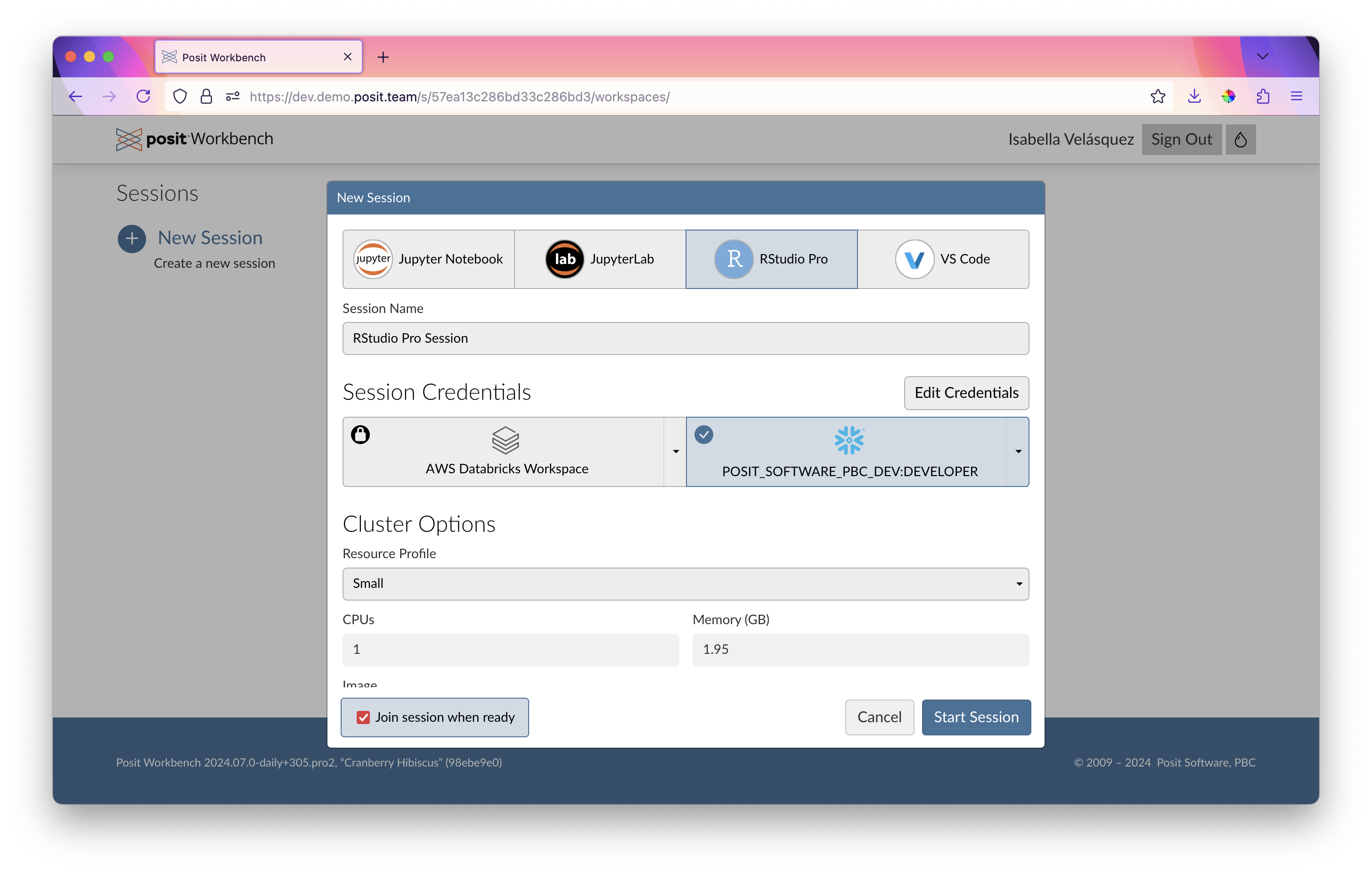
In this walkthrough, we connect to Snowflake using Posit Workbench on Snowpark Container Services (SPCS) to work with a sample of the lendingclub dataset. We use Snowflake compute to retrieve 2,000 rows, select the target feature, and perform feature engineering steps to train the model, which is then saved to Posit Connect using pins. With the orbital package, we then convert the trained model into an orbital object. Orbital translates the model and feature engineering steps into Snowflake SQL so that the inference can be performed directly on Snowflake compute. With a few dplyr commands, we can then transform this process into a Snowflake View that can be accessed by other Snowflake users.
- Connecting to Snowflake on Posit Workbench
- Running predictions with tidymodels
- Converting tidymodels workflows to Snowflake SQL with orbital
- Deploying a model as a Snowflake View
- Refitting models in Snowflake using Posit Connect
Connecting to Snowflake on Posit Workbench
A few months ago, we announced the Snowflake Native Posit Workbench App. The app allows users to develop in their preferred Integrated Development Environments (IDE) directly within Posit Workbench, alongside their data, while maintaining Snowflake’s security and governance protocols. With this setup, Posit Workbench users can log in and access their Snowflake resources seamlessly via SSO, ensuring secure and integrated data workflows.
An ODBC connection using the odbc::snowflake() function provides direct access to Snowflake data from within our R script without the need for additional configuration. We can connect to our desired warehouse, database, and schema of interest, such as the one storing the LendingClub data.
Important
If you’re running this for the first time, you may run into namespacing errors in Connect or permissioning errors in Snowflake. That means someone has already run this with the same model_name – to run this flawlessly, pick a new model_name below.
library(odbc)
library(DBI)
library(dbplyr)
library(dplyr)
library(glue)
library(arrow)
library(stringr)

con <- dbConnect(
  odbc::snowflake(),
  warehouse = "DEFAULT_WH",
  database = "LENDING_CLUB",
  schema = "PUBLIC"
)

model_name <- "interest_rate_prediction_blog"
Within RStudio Pro on Posit Workbench, we can get a quick and interactive view of our data by clicking on the table in the Connections pane:
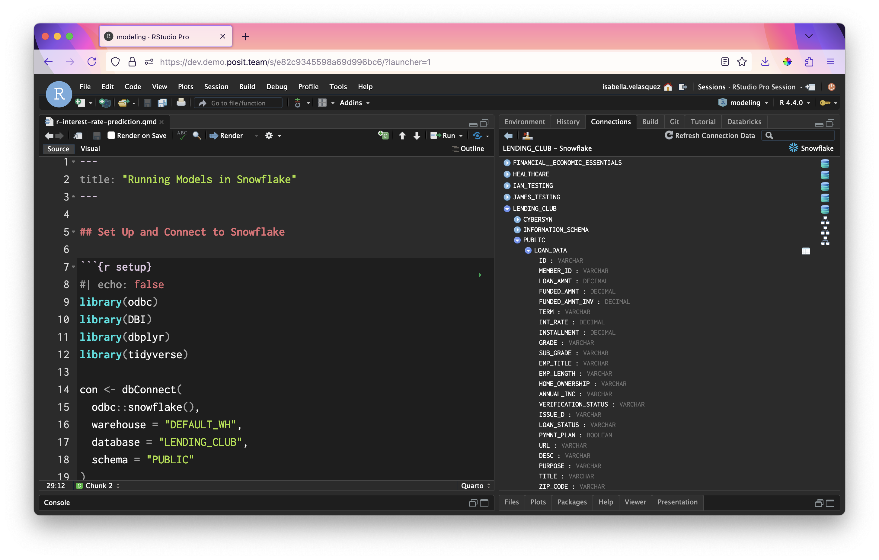
With this connection, we can create an object named lendingclub_dat that refers to our table in Snowflake. Let’s load and preview a sample of the data, lendingclub_sample.
lendingclub_dat <- con |> tbl("LOAN_DATA") |>
  mutate(ISSUE_YEAR = as.integer(str_sub(ISSUE_D, start = 5)),
         ISSUE_MONTH = as.integer(
           case_match(
             str_sub(ISSUE_D, end = 3),
             "Jan" ~ 1,
             "Feb" ~ 2,
             "Mar" ~ 3,
             "Apr" ~ 4,
             "May" ~ 5,
             "Jun" ~ 6,
             "Jul" ~ 7,
             "Aug" ~ 8,
             "Sep" ~ 9,
             "Oct" ~ 10,
             "Nov" ~ 11,
             "Dec" ~ 12
           )
         ))

lendingclub_sample <- lendingclub_dat |>
  filter(ISSUE_YEAR == 2016) |>
  slice_sample(n = 5000)

lendingclub_sample |>
  head()
# Source: SQL [6 x 153]
# Database: Snowflake 8.37.1[@Snowflake/LENDING_CLUB]
ID MEMBER_ID LOAN_AMNT FUNDED_AMNT FUNDED_AMNT_INV TERM INT_RATE
<chr> <chr> <dbl> <dbl> <dbl> <chr> <dbl>
1 83829525 <NA> 17000 17000 17000 36 months 8.99
2 74646059 <NA> 8000 8000 8000 36 months 7.89
3 91142172 <NA> 1000 1000 1000 36 months 9.49
4 76022991 <NA> 10000 10000 10000 36 months 8.39
5 91611365 <NA> 20000 20000 20000 60 months 10.5
6 81534155 <NA> 20000 20000 20000 60 months 15.6
# ℹ 146 more variables: INSTALLMENT <dbl>, GRADE <chr>, SUB_GRADE <chr>,
# EMP_TITLE <chr>, EMP_LENGTH <chr>, HOME_OWNERSHIP <chr>, ANNUAL_INC <chr>,
# VERIFICATION_STATUS <chr>, ISSUE_D <chr>, LOAN_STATUS <chr>,
# PYMNT_PLAN <lgl>, URL <chr>, DESC <chr>, PURPOSE <chr>, TITLE <chr>,
# ZIP_CODE <chr>, ADDR_STATE <chr>, DTI <dbl>, DELINQ_2YRS <dbl>,
# EARLIEST_CR_LINE <chr>, FICO_RANGE_LOW <dbl>, FICO_RANGE_HIGH <dbl>,
# INQ_LAST_6MTHS <dbl>, MTHS_SINCE_LAST_DELINQ <dbl>, …Running predictions with tidymodels
From here, we can select the columns of interest for our model. We’d typically find these columns using exploratory data analysis techniques. To keep this brief, we’ve omitted this step and skipped right to the features we know work. Then, we download the data locally with collect().
lendingclub_prep <- lendingclub_sample |>
  select(INT_RATE, TERM, BC_UTIL, BC_OPEN_TO_BUY, ALL_UTIL) |>
  mutate(INT_RATE = as.numeric(str_remove(INT_RATE, "%"))) |>
  filter(!if_any(everything(), is.na)) |>
  collect()
Next, we can run the following code to create a tidymodels workflow that runs the preprocessing steps along with a linear regression model.
library(tidymodels)

lendingclub_rec <- recipe(INT_RATE ~ ., data = lendingclub_prep) |>
  step_mutate(TERM = (TERM == "60 months")) |>
  step_mutate(across(!TERM, as.numeric)) |>
  step_normalize(all_numeric_predictors()) |>
  step_impute_mean(all_of(c("BC_OPEN_TO_BUY", "BC_UTIL"))) |>
  step_filter(!if_any(everything(), is.na))

lendingclub_lr <- linear_reg()

lendingclub_wf <- workflow() |>
  add_model(lendingclub_lr) |>
  add_recipe(lendingclub_rec)

lendingclub_wf
══ Workflow ════════════════════════════════════════════════════════════════════
Preprocessor: Recipe
Model: linear_reg()
── Preprocessor ────────────────────────────────────────────────────────────────
5 Recipe Steps
• step_mutate()
• step_mutate()
• step_normalize()
• step_impute_mean()
• step_filter()
── Model ───────────────────────────────────────────────────────────────────────
Linear Regression Model Specification (regression)
Computational engine: lm We fit the model from the lendingclub_wf workflow in a variable called lendingclub_fit. Then, we compute our model statistics: rmse, mae, and rsq.
lendingclub_fit <- lendingclub_wf |>
  fit(data = lendingclub_prep)

lendingclub_metric_set <- metric_set(rmse, mae, rsq)

lendingclub_metrics <- lendingclub_fit |>
  augment(lendingclub_prep) |>
  lendingclub_metric_set(truth = INT_RATE, estimate = .pred)

lendingclub_metrics
# A tibble: 3 × 3
.metric .estimator .estimate
<chr> <chr> <dbl>
1 rmse standard 4.39
2 mae standard 3.44
3 rsq standard 0.225Now, we register the model using the vetiver package. This step saves the lendingclub_fit fitted model on a “board” for future use using the pins package. In this example, the board is Posit Connect. Vetiver allows for a wide range of MLOps actions – in this case, pinning the model to Posit Connect allows us to version the model and track the performance of different model versions over time.
library(vetiver)
library(rsconnect)
library(pins)

board <- board_connect()

v <- vetiver_model(lendingclub_fit,
                   model_name,
                   metadata = list(metrics = lendingclub_metrics))

board |> vetiver_pin_write(v)
Let’s identify the active model version. The pins package version controls previously uploaded pins so that past versions can be retrieved and reused. It also enables us to check for the latest or the active version.
board <- board_connect()Connecting to Posit Connect 2024.08.0 at <https://pub.demo.posit.team>model_versions <- board |>
pin_versions(glue("{board$account}/{model_name}"))
model_versions# A tibble: 4 × 4
version created active size
<chr> <dttm> <lgl> <dbl>
1 634 2024-10-03 15:27:00 TRUE 278882
2 630 2024-10-03 14:18:00 FALSE 278613
3 626 2024-10-02 21:03:00 FALSE 278647
4 624 2024-10-02 20:52:00 FALSE 279283Let’s save the active model version number — we’re going to need it later!
model_version <- model_versions |>
  filter(active) |>
  pull(version)

model_version
[1] "634"In this case, our active model is version 634.
We can measure the performance of the model using vetiver_compute_metrics(), first adding the predictions with the augment() function.
original_metrics <- lendingclub_fit |>
  augment(lendingclub_prep) |>
  mutate(date_obs = lubridate::today()) |>
  vetiver_compute_metrics(date_obs, "day", INT_RATE, .pred)

original_metrics
# A tibble: 3 × 5
.index .n .metric .estimator .estimate
<date> <int> <chr> <chr> <dbl>
1 2024-10-03 4940 rmse standard 4.39
2 2024-10-03 4940 rsq standard 0.225
3 2024-10-03 4940 mae standard 3.44 Converting tidymodels workflows to Snowflake SQL with orbital
We can now use the orbital package to transform the lendingclub_fit model into an orbital object. This conversion allows the tidymodels workflow to be executed directly on Snowflake.
library(orbital)
library(tidypredict)

orbital_obj <- orbital(lendingclub_fit)
orbital_obj
── orbital Object ──────────────────────────────────────────────────────────────
• TERM = (TERM == "60 months")
• BC_UTIL = (BC_UTIL - 58.56933) / 28.12647
• BC_OPEN_TO_BUY = (BC_OPEN_TO_BUY - 10459.8) / 15135.56
• ALL_UTIL = (ALL_UTIL - 60.367) / 20.30032
• BC_OPEN_TO_BUY = dplyr::if_else(is.na(BC_OPEN_TO_BUY), 5.152585e-17, BC ...
• BC_UTIL = dplyr::if_else(is.na(BC_UTIL), 1.049699e-16, BC_UTIL)
• .pred = 11.98086 + (ifelse(TERM == "TRUE", 1, 0) * 4.276453) + (BC_UTIL ...
────────────────────────────────────────────────────────────────────────────────
7 equations in total.We can inspect the model’s full Snowflake SQL syntax. Note that this includes both the preprocessing steps we defined above as well as the coefficients required to fit the linear model.
sql_predictor <- orbital_sql(orbital_obj, con)
sql_predictor
<SQL> ("TERM" = '60 months') AS TERM
<SQL> ("BC_UTIL" - 58.5693319838057) / 28.1264677961075 AS BC_UTIL
<SQL> ("BC_OPEN_TO_BUY" - 10459.8006072874) / 15135.5559905029 AS BC_OPEN_TO_BUY
<SQL> ("ALL_UTIL" - 60.367004048583) / 20.3003247059405 AS ALL_UTIL
<SQL> CASE WHEN (("BC_OPEN_TO_BUY" IS NULL)) THEN 5.15258522982901e-17 WHEN NOT (("BC_OPEN_TO_BUY" IS NULL)) THEN "BC_OPEN_TO_BUY" END AS BC_OPEN_TO_BUY
<SQL> CASE WHEN (("BC_UTIL" IS NULL)) THEN 1.04969908440208e-16 WHEN NOT (("BC_UTIL" IS NULL)) THEN "BC_UTIL" END AS BC_UTIL
<SQL> (((11.9808586664457 + (CASE WHEN ("TERM" = 'TRUE') THEN 1.0 WHEN NOT ("TERM" = 'TRUE') THEN 0.0 END * 4.27645329075645)) + ("BC_UTIL" * 0.158913569656065)) + ("BC_OPEN_TO_BUY" * -0.770493364808141)) + ("ALL_UTIL" * 0.801915544019693) AS .predWith the model converted, we can run predictions directly in Snowflake, saving the results to a temporary table.
preds <- predict(orbital_obj, lendingclub_dat) |>
  compute(name = "LENDING_CLUB_PREDICTIONS_TEMP")

preds |> filter(!is.na(.pred))
# Source: SQL [?? x 1]
# Database: Snowflake 8.37.1[@Snowflake/LENDING_CLUB]
.pred
<dbl>
1 11.3
2 8.15
3 16.8
4 13.1
5 17.4
6 13.3
7 13.3
8 11.3
9 11.5
10 11.5
# ℹ more rowsWe can also visualize the predictions by plotting a histogram.
library(ggplot2)

lendingclub_16 <- lendingclub_dat |>
  filter(ISSUE_YEAR == 2016)

orbital_obj |>
  predict(lendingclub_16) |>
  collect() |>
  ggplot() +
  geom_histogram(aes(.pred))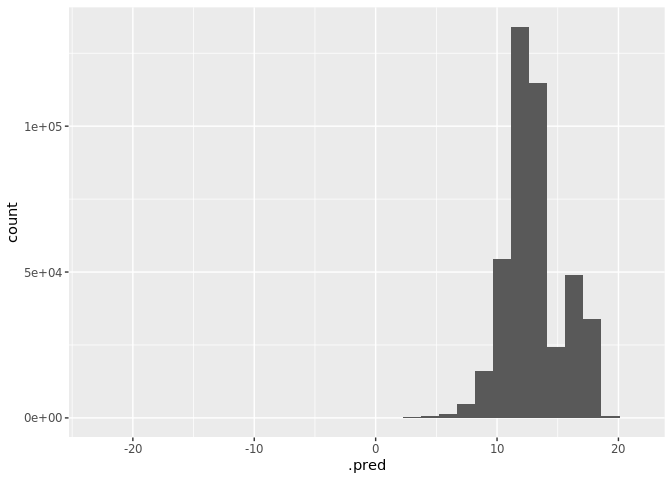
Next, we can count the number of predictions generated.
preds |> count()# Source: SQL [1 x 1]
# Database: Snowflake 8.37.1[@Snowflake/LENDING_CLUB]
n
<dbl>
1 2260702The result? 2,260,702 predictions in just 2.5 seconds — an incredible speed, thanks to Snowflake’s compute power!
Real-time inference on Posit Connect
What if we need real-time inference instead of batch processing? This is easy – deploy the model as an API on Posit Connect!
First, deploy the model to Posit Connect with a distinctive name.
vetiver_deploy_rsconnect(board, glue("{board$account}/{model_name}"))Deploying a model as a Snowflake View
A Snowflake View allows query results to be accessed as if they were a table, but the query only runs when the view is called. Views can be included in Snowflake’s Optimized Query plans, often making them more efficient than stored procedures.
Here, we deploy our model as a Snowflake View by adding a predictions column to the table. We select only the prediction and ID columns, then translate the dbplyr tbl into a SQL query string.
# Add predictions column to table
res <- dplyr::mutate(lendingclub_dat, !!!orbital_inline(orbital_obj))

# Select only the prediction column and the ID column
pred_name <- ".pred"
res <- dplyr::select(res, dplyr::any_of(c("ID", pred_name)))

# Translate the dbplyr `tbl` into a SQL query string
generated_sql <- remote_query(res)
Then, we convert the generated SQL into a Snowflake View. We’ll start by creating a “versioned” view, linked to the version of the model we just fit. We’ll use the view associated with this model version to generate predictions.
versioned_view_name <-
  glue("{model_name}_v{model_version}")

snowflake_view_statement <-
  glue::glue_sql("CREATE OR REPLACE VIEW {`versioned_view_name`} AS ",
                 generated_sql,
                 .con = con)

# NOTE: Uncomment the following line to see the whole Snowflake View creation statement.
# snowflake_view_statement
Finally, we dispatch our view creation statement to Snowflake (the 0 is to be expected. dbExecute returns the number of affected rows. Since we created a view, the number affected is zero).
con |>
  DBI::dbExecute(snowflake_view_statement)
[1] 0Next, we’ll create a “main” view that stays in sync with the latest model version. This ensures that downstream projects can always reference this view and pull the most up-to-date predictions.
main_view_name <- glue::glue("{model_name}_latest")

main_view_statement <- glue::glue_sql(
  "CREATE OR REPLACE VIEW {`main_view_name`} AS ",
  "SELECT * FROM {`versioned_view_name`}",
  .con = con
)

con |>
  DBI::dbExecute(main_view_statement)
[1] 0Now, let’s try our view!
con |>
  tbl(main_view_name) |>
  head() |>
  collect()
# A tibble: 6 × 2
ID .pred
<chr> <dbl>
1 68407277 11.3
2 68355089 8.15
3 68341763 16.8
4 66310712 13.1
5 68476807 17.4
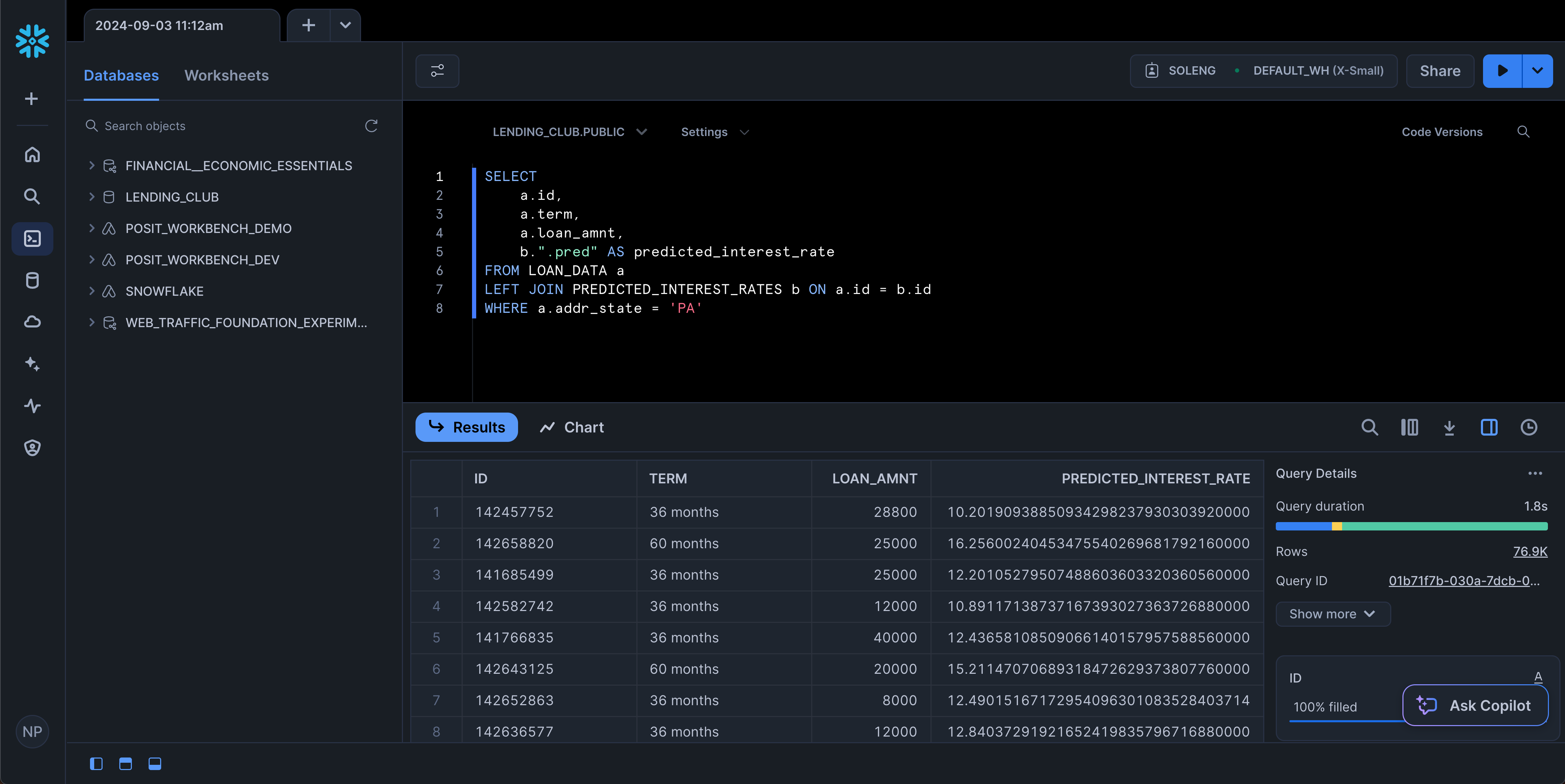
6 68426831 13.3 You can now access the view from any service that can access Snowflake, including the SnowSight UI!
Refitting models in Snowflake using Posit Connect
Once a model is deployed, it is important to monitor its statistical performance over time. As new data comes in over time, model performance can “drift” and degrade. We can refit the model periodically and store the best-performing version as a pin on Connect. The code below monitors model performance, refits the model as needed, and compares RMSE values. If the new model performs better, it replaces the old one and updates Snowflake views accordingly.
Here, we authenticate our Snowflake access.
# Use SSH key if on Connect, otherwise use managed credentials
if (Sys.getenv("RSTUDIO_PRODUCT") == "CONNECT") {
  # Grab base64-encoded SHH key from environment variable and cache as tempfile
  cached_key <- tempfile()
  readr::write_file(openssl::base64_decode(Sys.getenv("SNOWFLAKE_SSH_KEY")), file = cached_key)

  # The ambient credential feature in odbc::snowflake() causes unexpected overwrites, so we'll use the base Snowflake driver
  con <- dbConnect(
    odbc::odbc(),
    driver = "Snowflake",
    server = paste0(
      Sys.getenv("SNOWFLAKE_ACCOUNT"),
      ".snowflakecomputing.com"
    ),
    uid = "SVC_SOLENG",
    role = "SOLENG",
    warehouse = "DEFAULT_WH",
    database = "LENDING_CLUB",
    schema = "PUBLIC",
    # Settings to set Snowflake key-pair auth
    authenticator = "SNOWFLAKE_JWT",
    PRIV_KEY_FILE = cached_key
  )

} else {
  con <- dbConnect(
    odbc::snowflake(),
    warehouse = "DEFAULT_WH",
    database = "LENDING_CLUB",
    schema = "PUBLIC"
  )

}
Let’s join our original dataset, lendingclub_raw, with the versioned dataset containing predictions, lendingclub_predictions, and save the join in the existing_predictions object.
lendingclub_raw <- con |> tbl("LOAN_DATA") |>
  mutate(ISSUE_YEAR = as.integer(str_sub(ISSUE_D, start = 5)),
         ISSUE_MONTH = as.integer(case_match(
           str_sub(ISSUE_D, end = 3),
          "Jan" ~ 1,
          "Feb" ~ 2,
          "Mar" ~ 3,
          "Apr" ~ 4,
          "May" ~ 5,
          "Jun" ~ 6,
          "Jul" ~ 7,
          "Aug" ~ 8,
          "Sep" ~ 9,
          "Oct" ~ 10,
          "Nov" ~ 11,
          "Dec" ~ 12
           ))
         ) |>
  filter(ISSUE_YEAR >= 2016, ISSUE_YEAR < 2018)

lendingclub_predictions <- con |>
  tbl(glue("{model_name}_v{model_version}"))

existing_predictions <- lendingclub_raw |>
  left_join(lendingclub_predictions, by = "ID") |>
  select(ID, ISSUE_YEAR, ISSUE_MONTH, INT_RATE, .pred) |>
  collect()

existing_predictions
# A tibble: 877,989 × 5
ID ISSUE_YEAR ISSUE_MONTH INT_RATE .pred
<chr> <dbl> <dbl> <dbl> <dbl>
1 113026220 2017 7 9.44 8.45
2 112737437 2017 7 16.0 12.2
3 112728535 2017 7 9.44 8.89
4 112135359 2017 7 21.4 15.4
5 112380195 2017 7 13.6 10.7
6 112465977 2017 7 19.0 17.5
7 112062878 2017 7 19.0 16.6
8 112753060 2017 7 9.44 12.4
9 112712008 2017 7 13.6 13.3
10 112733143 2017 7 10.9 4.95
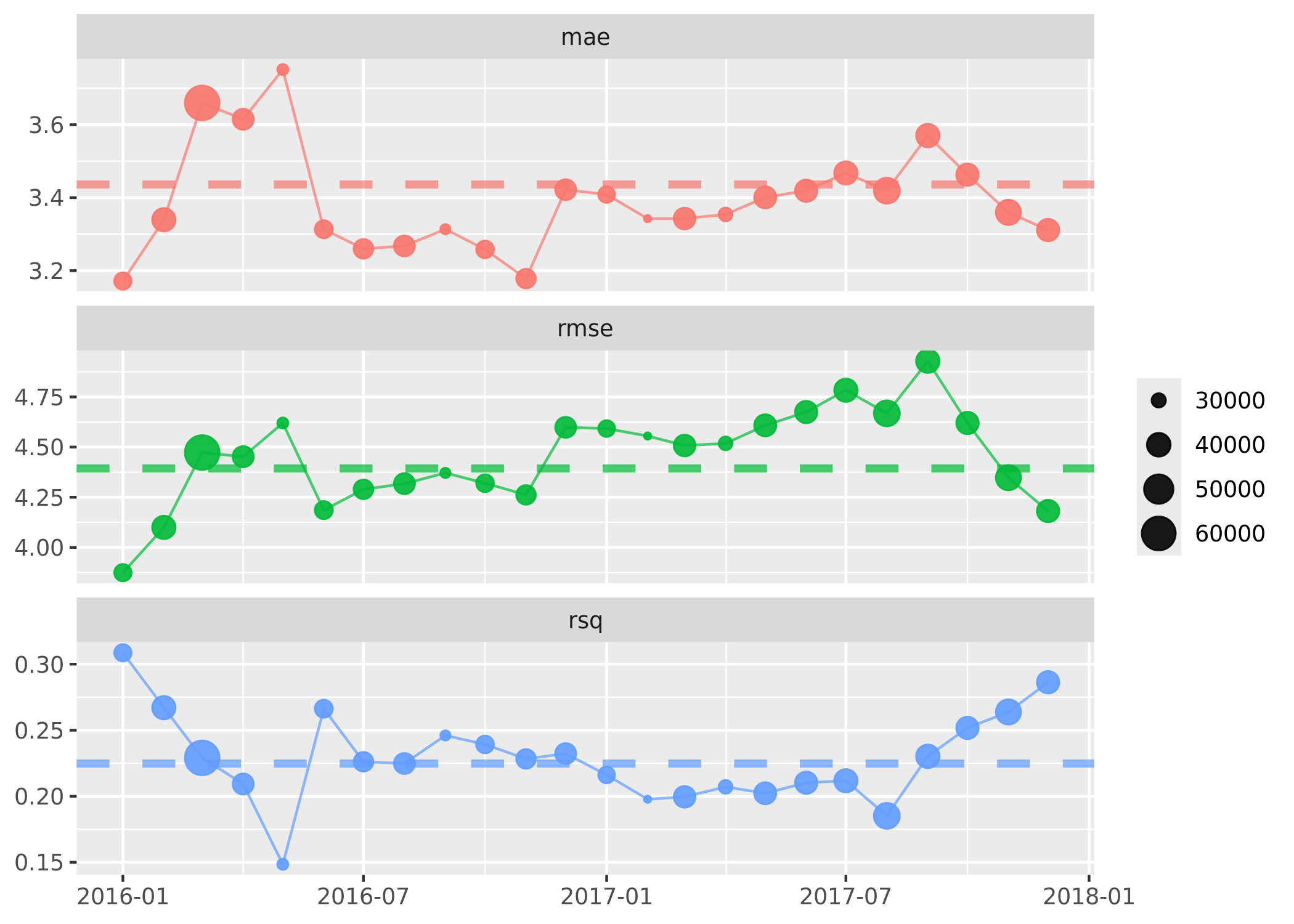
# ℹ 877,979 more rowsMonitoring Model Performance Over Time
By retrieving our pinned model from Connect, we can extract the metrics from the latest model into extracted_metrics. We then append these metrics to existing_predictions so we can compare summary statistics over time.
# Extract the metrics from our last model run
extracted_metrics <- board |>
    pin_meta(glue("{board$account}/{model_name}")) %>%
    pluck("user", "metrics") %>%
    as_tibble()

metrics <- existing_predictions |>
  mutate(date = lubridate::ymd(glue(
    "{ISSUE_YEAR}-{str_pad(ISSUE_MONTH, 2, pad=0)}-01"
  ))) |>
  arrange(date) |>
  vetiver_compute_metrics(date, "month", INT_RATE, .pred)

metrics |>
  vetiver_plot_metrics() +
  geom_hline(
    aes(yintercept = .estimate, color = .metric),
    data = extracted_metrics,
    linewidth = 1.5,
    alpha = 0.7,
    lty = 2
  )
Retraining our Model on New Data
Let’s take a sample of 20,000 rows to refit the model.
lendingclub_prep <- lendingclub_dat |>
  slice_sample(n = 20000) |>
  select(INT_RATE, TERM, BC_UTIL, BC_OPEN_TO_BUY, ALL_UTIL) |>
  mutate(INT_RATE = as.numeric(stringr::str_remove(INT_RATE, "%"))) |>
  filter(!if_any(everything(), is.na)) |>
  collect()
Now, let’s refit the model using the new data and see if it shows any improvement!
lendingclub_rec <- recipe(INT_RATE ~ ., data = lendingclub_prep) |>
  step_mutate(TERM = (TERM == "60 months")) |>
  step_mutate(across(!TERM, as.numeric)) |>
  step_normalize(all_numeric_predictors()) |>
  step_impute_mean(all_of(c("BC_OPEN_TO_BUY", "BC_UTIL"))) |>
  step_filter(!if_any(everything(), is.na))

lendingclub_lr <- linear_reg()

lendingclub_wf <- workflow() |>
  add_model(lendingclub_lr) |>
  add_recipe(lendingclub_rec)

lendingclub_fit <- lendingclub_wf |>
  fit(data = lendingclub_prep)
Recalculate the model’s statistics to find out.
lendingclub_metric_set <- metric_set(rmse, mae, rsq)

lendingclub_metrics <- lendingclub_fit |>
  augment(lendingclub_prep) |>
  lendingclub_metric_set(truth = INT_RATE, estimate = .pred)

lendingclub_metrics
# A tibble: 3 × 3
.metric .estimator .estimate
<chr> <chr> <dbl>
1 rmse standard 4.49
2 mae standard 3.47
3 rsq standard 0.230We’ll select the best model by choosing the one with the lowest RMSE. The callout note will state whether or not the model will be updated. Note that all these code blocks are wrapped in if (update_model){...}, which uses the update_model flag set in the previous code chunk to control whether the code is executed.
old_rmse <- extracted_metrics |>
  filter(.metric == "rmse") |>
  pull(.estimate) |>
  round(digits = 4)

new_rmse <- lendingclub_metrics |>
  filter(.metric == "rmse") |>
  pull(.estimate) |>
  round(digits = 4)

if (old_rmse > new_rmse) {
  update_model <- TRUE
  cat(
    "\n::: {.callout-tip}",
    "## Model Will Be Updated",
    glue(
      "New Model RMSE of {new_rmse} is lower than the Previous RMSE of {old_rmse}. Updating model in Snowflake!"
    ),
    ":::\n",
    sep = "\n"
  )
} else {
  update_model <- FALSE
  cat(
    "\n::: {.callout-important}",
    "## Model Will Not Be Updated",
    glue(
      "New Model RMSE of {new_rmse} is higher than the Previous RMSE of {old_rmse}. No updates will occur. Please note that the cells following this block will not be evaluated."
    ),
    ":::\n",
    sep = "\n"
  )
}
[!IMPORTANT]
Model Will Not Be Updated
New Model RMSE of 4.4896 is higher than the Previous RMSE of 4.3934. No updates will occur. Please note that the cells following this block will not be evaluated.
Finally, we pin the new model version (if applicable) to Connect so it’s stored and available for future use.
if (update_model) {
  v <- vetiver_model(lendingclub_fit,
                     model_name,
                     metadata = list(metrics = lendingclub_metrics))

  board |>
    vetiver_pin_write(v)

  model_versions <- board |>
    pin_versions(glue("{board$account}/{model_name}"))

  model_version <- model_versions |>
    filter(active) |>
    pull(version)
}
If the model is updated, we also create a corresponding orbital object to reflect the changes.
if (update_model){

  library(orbital)
  library(tidypredict)

  orbital_obj <- orbital(lendingclub_fit)

  ## Add predictions column to table

  res <- tbl(con, "LOAN_DATA") |>
    mutate(!!!orbital_inline(orbital_obj))

  # Select only the prediction column and the ID column
  pred_name <- ".pred"
  res <- select(res, any_of(c("ID", pred_name)))

  # Translate the dbplyr `tbl` into a sql query string
  generated_sql <- remote_query(res)
}
Translate the generated SQL into a Snowflake View. We will begin by creating a “versioned” view that is linked to the version of the model we just fitted.
if (update_model) {

  versioned_view_name <- glue("{model_name}_v{model_version}")
  snowflake_view_statement <-
    glue::glue_sql("CREATE OR REPLACE VIEW {`versioned_view_name`} AS ",
                   generated_sql,
                   .con = con)

  con |> DBI::dbExecute(snowflake_view_statement)

}
Next, we’ll create a “main” view that will be kept up-to-date with the latest model version. This ensures that downstream projects can always reference this view and receive the most current updates.
if (update_model){

  main_view_name <- glue("{model_name}_latest")
  main_view_statement <-
    glue::glue_sql(
      "CREATE OR REPLACE VIEW {`main_view_name`} AS ",
      "SELECT * FROM {`versioned_view_name`}",
      .con = con
  )

  con |> DBI::dbExecute(main_view_statement)

}
Regularly updating our models and creating versioned views ensures that downstream projects benefit from the latest predictions and insights – and it’s all integrated entirely within the Posit Team ecosystem.
Learn more about machine learning operations with Posit
With the orbital package, we can take advantage of the power of tidymodels with the scalable and performant environment of a database backend without the need to rewrite code from R into another language or deal with running an R process in the database platform.
For Snowflake users, we can leverage Snowflake’s compute capabilities and translate models into Snowflake SQL for rapid, scalable inference without additional dependencies. Then, we can deploy models as Snowflake Views and orchestrate workflows through Posit Connect for machine learning operations.
Learn more:
Footnotes
Please note that not all models or recipes are currently supported. There’s room for expansion, and the tidymodels team is actively listening for community feedback and requests to guide future updates. Share yours here.↩︎

Isabella Velásquez
Related Content

Don't bring a spreadsheet to a data fight

Snowflake Native Apps vs. Connected Apps for financial services
